Probability tools: getting ready to read the RAG formula
This lesson builds five tools: conditional probability, the chain rule, marginalization, softmax and loss. Lesson 5's RAG formula is made of exactly these five. That formula combines two kinds of numbers. In lesson 1, after reading the queue log, the LLM gave Thursday a of 0.81. In lesson 3, the retriever gave the course's long FAQ page a of 1.56.
These two numbers do not combine directly. 1.56 cannot be a probability, because a probability is never larger than 1. And 0.81 is not the chance of the whole answer, only of its first token. The formula in lesson 5 combines them like this: p(y|x) ≈ ∑ p(z|x) · p(y|x, z), where p(z|x) ∝ exp(d(z)⊤q(x)), and training makes ∑ −log p(y|x) small. In step 5 you will run this whole formula by hand.
The ladder for this lesson
The ladder has 5 steps. Under each step you can see what you will be able to do after it.
Conditional probability and the chain ruleWork out a probability like p(full | Tuesday) from counts, and build the probability of a whole answer from its tokens' probabilities.
The whole RAG formula by handWork out every part of the formula from your own numbers, and read Stanford's RAG slide.
What you need first: Lesson 1 (probability, token, next-token prediction, training) and Lesson 3 (vector, dot product, ∑). If you already know a step, skip to the next one. A word with a dotted underline and ▾ opens its definition when you click it.
1Conditional probability and the chain rule: a chance that depends on what you know
What comes after the “|” is already known
A conditional probability is the chance of something when something else is already known. It is written p(A | B) and read “the probability of A, given B”. Every probability in the RAG formula has this vertical bar “|” inside it, so start by seeing what it means with numbers.
Over the last 20 weeks there were 40 office hour sessions, 20 on Tuesday and 20 on Thursday. Call a session “full” if more than 10 students were waiting. my numbers
Full
Empty
Total
Tuesday
16
4
20
Thursday
2
18
20
Total
18
22
40
If you do not know the day, count all 40 sessions. 18 of them were full, so p(full) = 18 ÷ 40 = 0.45. Now suppose you know today is Tuesday. Then you count only the Tuesday row, where 16 of 20 were full, so p(full | Tuesday) = 16 ÷ 20 = 0.80. If you know it is Thursday, p(full | Thursday) = 2 ÷ 20 = 0.10. As soon as the day is known, the chance moves from 0.45 to 0.80 or to 0.10.
p(A | B) = cases with both A and Bcases with B
For Tuesday, the top is 16, the full Tuesdays, and the bottom is 20, all Tuesdays.
Next-token prediction from lesson 1 is also a conditional probability. There the prompt was known, and Thursday had probability 0.21. When the queue log was added to the prompt, what was known changed, and the same probability became 0.81.
You can now read both pieces of the formula. p(z|x) is the probability of passage z, given the question x. p(y|x, z) is the probability of the answer y, given both the question x and the passage z. Read the comma after the “|” as “and”.
The probability of a whole answer: the chain rule
An LLM writes one token at a time, and each token has its own probability. But p(y|x, z) in the formula is the probability of the whole answer y, such as Thursday morning. The rule for turning three token probabilities into one probability is already visible in the table above.
In the table, Tuesday and full happened together 16 times out of 40, which is 0.40. The same number also comes out in two steps. First take the chance of Tuesday: p(Tuesday) = 20 ÷ 40 = 0.5. Then take the chance of full, given Tuesday: p(full | Tuesday) = 0.8. Their product is 0.5 × 0.8 = 0.40.
p(A and B) = p(A) × p(B | A)
The probability of two things together is the probability of the first, times the probability of the second given the first. This rule is the . Lesson 12 has a different rule with the same name, about rates, so call this one the chain rule for probabilities.
For the tokens of an answer, this rule runs again and again. The first token is Thursday, with probability 0.21. Once Thursday is written, morning has probability 0.31, and then the full stop has 0.71. The probability of the whole answer is the product of the three. For the two answers from the widget in lesson 1, it looks like this:
Answer
Probability of each token
Probability of the whole answer
Thursday morning.
0.21 × 0.31 × 0.71
0.046
Wednesday afternoon.
0.34 × 0.46 × 0.71
0.111
For an answer of n tokens, the same product is written with . ∏ means multiply everything over the range written below it, just as ∑ means add everything. yi is the i-th token of the answer, and after the “|” in its probability come the question x and all the tokens before it:
p(y | x) = ∏i = 1 … n p(yi | x, y1 … yi−1)
In our answer n = 3: y1 = Thursday, y2 = morning and y3 = the full stop. In the probability of y2, the question and Thursday come after the “|”. The whole product is 0.21 × 0.31 × 0.71 = 0.046.
This product has a problem. Every probability is below 1, so the result shrinks with every multiplication. With 20 tokens of probability 0.5 each, the whole answer gets 0.520 = 0.00000095. The ln in step 4 solves exactly this problem.
Think first
An answer has 4 tokens with probabilities 0.9, 0.8, 0.5 and 0.9. What is the probability of the whole answer?
Show the answer
0.9 × 0.8 = 0.72, then 0.72 × 0.5 = 0.36, and then 0.36 × 0.9 = 0.324. The other three tokens are at 0.8 or above, yet the single 0.5 token halved the probability of the whole answer.
2Marginalization: when you do not know which case is true
Marginalization is the way to get a total probability when you do not know which case is true. Multiply each case's probability by the chance within that case, then add up the products. We will call a case's probability its weight.
This is exactly the situation in RAG. The retriever brings several passages, and the system does not know in advance which passage is right. With the queue log, the LLM will give Thursday 9am a high probability, and with the old forum post a low one. The system has to turn these into a single probability.
First look at the same situation with office hours, where the numbers are small. A student goes on Tuesday half the weeks and on Thursday the other half, so p(Tuesday) = 0.5 and p(Thursday) = 0.5. The chance of a full session on each day is known from step 1: 0.8 and 0.1. You just do not know which day the student will go today.
Case z
Weight p(z)
p(full | z)
Product
Tuesday
0.5
0.8
0.40
Thursday
0.5
0.1
?
Sum = p(full)
?
Work out the Thursday row
What is the Thursday product, and what is the total p(full)? If the student goes on Thursday 90% of the time, what is the total chance?
Show the answer
Thursday: 0.5 × 0.1 = 0.05. The sum is 0.40 + 0.05 = 0.45, the same number step 1 got by counting directly, 18 ÷ 40.
With Thursday 90% of the time: 0.1 × 0.8 + 0.9 × 0.1 = 0.08 + 0.09 = 0.17. The chance on each day stayed the same, only the weights changed, and the total went from 0.45 to 0.17.
This method is called . It is correct only when the cases do not overlap and their weights add up to 1. Both hold here, because on a given day the student goes either on Tuesday or on Thursday, and 0.5 + 0.5 = 1.
p(A) = ∑z p(z) × p(A | z)
z is a case, here Tuesday or Thursday. p(z) is its weight, 0.5 and 0.5, and p(A | z) is the chance of full in that case, 0.8 and 0.1. adds over all the cases, here 0.40 + 0.05, and the result is p(A) = 0.45.
The RAG formula in lesson 5 is exactly this. There a case z is a passage, and its weight is the retriever's confidence p(z|x). The probability of the answer with each passage is p(y|x, z), the product of token probabilities from step 1.
The RAG formula has instead of “=”, which means “approximately equal”. RAG does not add up every passage, only the retriever's passages, the K passages with the highest scores. The other passages have very small weights, so the sum stays nearly the same.
One condition is still open. Every weight must lie between 0 and 1, and all the weights must add up to 1. The retriever's scores are not like that, so step 3 turns them into weights.
3Softmax: weights from the retriever's scores
Softmax turns a list of scores into a list of probabilities. It has two steps: take the exp of each score, then divide each exp by the sum of all the exps. First see why both steps are needed.
In lesson 3 the question when can I get help from a TA had a vector. The retriever took the of that vector with each passage's vector, multiplying the numbers in the same positions and adding the results. For the office hours page that was 0.8 × 0.9 + 0.2 × 0.1 = 0.74. The other scores were: syllabus 0.26, project page 0.32 and the course's long FAQ page 1.56.
These are not probabilities, because 1.56 is larger than 1, and the four add up to 2.88, not 1. Dividing each score by the sum of the four does not always work either, because a dot product can also be negative. That would give a negative share, and a probability is never negative.
So softmax first turns every score into a positive number, and it uses for that. exp(s) = es, where e is a fixed number, about 2.718. For example, exp(1) = 2.718 and exp(2) = e × e = 7.389. exp(0) = 1, because any number raised to the power 0 gives 1.
For a negative score, exp is still positive: exp(−1) = 1 ÷ e = 0.368. Whatever the score, exp is always above 0, and a larger score gives a much larger exp. One rule of exp will be useful later: adding 1 to a score multiplies its exp by e, because ea+1 = ea × e. Check: exp(2) = exp(1) × e = 2.7183 × 2.7183 = 7.389.
Now see the two steps of softmax on the scores 2.0, 1.0 and 0.1: my scores
Score s
exp(s)
Arithmetic
Probability
2.0
7.389
7.389 ÷ 11.212
0.659
1.0
2.718
2.718 ÷ 11.212
0.242
0.1
1.105
1.105 ÷ 11.212
0.099
Sum
11.212
1.000
The three exps add up to 11.212, and dividing each exp by that gives 0.659, 0.242 and 0.099. All three lie between 0 and 1 and add up to 1, so they can serve as weights. This whole method is called :
pi = exp(si)∑j exp(sj)
On top is the exp of score si, such as exp(2.0) = 7.389 in the first row. Below is the sum of the exps of all the scores, 11.212. So p1 = 7.389 ÷ 11.212 = 0.659.
Think first
Add 1 to every score, giving 3.0, 2.0 and 1.1. Will the probabilities go up, go down, or stay the same?
Show the answer
They stay the same: 0.659, 0.242 and 0.099. Adding 1 to a score multiplies each exp by e, as when exp(2.0) = 7.389 becomes exp(3.0) = 20.09. The top and the bottom are both multiplied by e, and the division cancels it. So softmax looks only at the differences between scores.
The formula in lesson 5 writes softmax in a short form:
p(z|x) ∝ exp(d(z)⊤q(x))
means “is proportional to”. You first take the exp for each passage, then divide them all by one and the same number, chosen so that they add up to 1. That number is the sum of all the exps, so the softmax division is hidden inside ∝.
is the dot product of the passage's vector and the question's vector. d(z) is the vector of passage z, and q(x) is the vector of question x. The ⊤ is only a way of writing it, and the arithmetic is the same as in lesson 3. For example, the office hours page [0.9, 0.1] and the question [0.8, 0.2] give 0.74.
Now the 1.56 from the start of the lesson can become a weight too. Softmax over the four scores from lesson 3 gives these weights: FAQ page 0.50, office hours page 0.22, project page 0.14 and syllabus 0.14. my arithmetic Softmax does not change the order, because a larger score always gives a larger exp. So the FAQ page is still on top, and softmax does not fix the long-vector problem from lesson 3.
Run softmax yourself
Change the scores of the three passages. The probabilities always add up to 1, and even with a negative score every probability stays above 0.
Passage
Score
exp(score)
Probability
4ln and loss: one number for the error
A loss is a number that says how far the model is from the right answer, and training makes this number small. In RAG the loss is built from the probability of the right answer, using ln. ln also solves the tiny-number problem from step 1, so look at ln first.
The , ln x, is the power you must raise e to in order to get x. So ln undoes exp: ln(ex) = x. For example, e1 = 2.718, so ln 2.718 = 1. And e0 = 1, so ln 1 = 0.
The ln of a number below 1 is negative, because getting such a number needs a negative power of e. For example, ln 0.1 = −2.303, because e−2.303 = 1 ÷ e2.303 = 1 ÷ 10 = 0.1.
The most useful rule of ln is this: ln(a × b) = ln a + ln b, so the ln of a product is the sum of the two lns. It comes from the rule of exp, because powers add when you multiply: e2 × e3 = e5. In numbers, 7.389 × 20.09 = 148.4, and e5 is also 148.4. ln gives exactly these powers, so ln 148.4 = 5 = 2 + 3 = ln 7.389 + ln 20.09.
For Thursday morning., this rule turns the product of three probabilities into the sum of three lns:
Check: e−3.074 = 0.046, the same product as before. For an answer of 20 tokens, instead of a tiny number like 0.520 = 0.00000095, you add ln 0.5 twenty times: 20 × (−0.693) = −13.86. my arithmetic
Now build the number for the error: = −ln p, where p is the probability the model gave the right answer. The minus sign in front makes the loss positive, because every probability below 1 has a negative ln. The table below shows how the loss grows as p falls:
Probability of the right answer
Loss = −ln p
Meaning
1
0
Fully sure and right. The loss cannot go lower.
0.9
0.105
Good
0.5
0.693
Half sure
0.1
2.303
Mostly wrong
0.01
4.605
Very wrong
At p = 0.9 the loss is 0.105, but at p = 0.1 it is 2.303, more than 20 times as much.
The probability the model gave the right answer is called the . The loss is minus the ln of it, so this loss is called the . If Thursday morning. is the right answer, its loss is −(−3.074) = 3.074.
In lesson 1, training changed the parameters a little. As a result, the probability of Thursday after Office hours are on went from 0.10 to 0.12. The loss fell from −ln 0.10 = 2.303 to −ln 0.12 = 2.120, a drop of 2.303 − 2.120 = 0.183.
Training data has many examples. Example j has a question xj and its right answer yj, and the total loss is the sum of the losses over all examples:
total loss = ∑j − log p(yj | xj)
Stanford's slide and the formula in lesson 5 write log, and they mean this ln.
The tells training which way, and by how much, to change each parameter so that the total loss goes down. In the Thursday example, training changed the parameters in the direction that raised the probability from 0.10 to 0.12 and lowered the loss by 0.183. How the gradient is worked out from numbers comes in lesson 12.
5The whole RAG formula by hand
Now the tools work together: softmax gives each passage a weight, marginalization gives the answer's total probability, and −ln gives its loss. Take the question from the start again: Which office hour is least crowded? The retriever brings two passages: the queue log and the old forum post. Their dot product scores are 1.0 and 0.0.
The LLM gives the right answer Thursday 9am a probability of 0.9 with the queue log, and 0.1 with the forum post. my numbers The whole calculation takes three steps:
Softmax (step 3): e1.0 = 2.718 and e0 = 1, which add up to 3.718. The queue log's weight is 2.718 ÷ 3.718 = 0.731, and the forum post's is 1 ÷ 3.718 = 0.269.
So the system is 0.685 sure that the answer is Thursday 9am, and the loss on this question is 0.378. If the retriever gives the queue log a higher score, its weight rises above 0.731, 0.685 rises too, and the loss falls. The formula holds the same three steps:
The dot product of the passage's and the question's vectors, here 1.0 and 0.0.
p(z|x)
The softmax weight, here 0.731 and 0.269.
p(y|x, z)
The probability of the whole answer with that passage, here 0.9 and 0.1.
∑ and ≈
The weighted sum over K = 2 passages, here 0.685.
−log p(y|x)
The loss for this question, here 0.378.
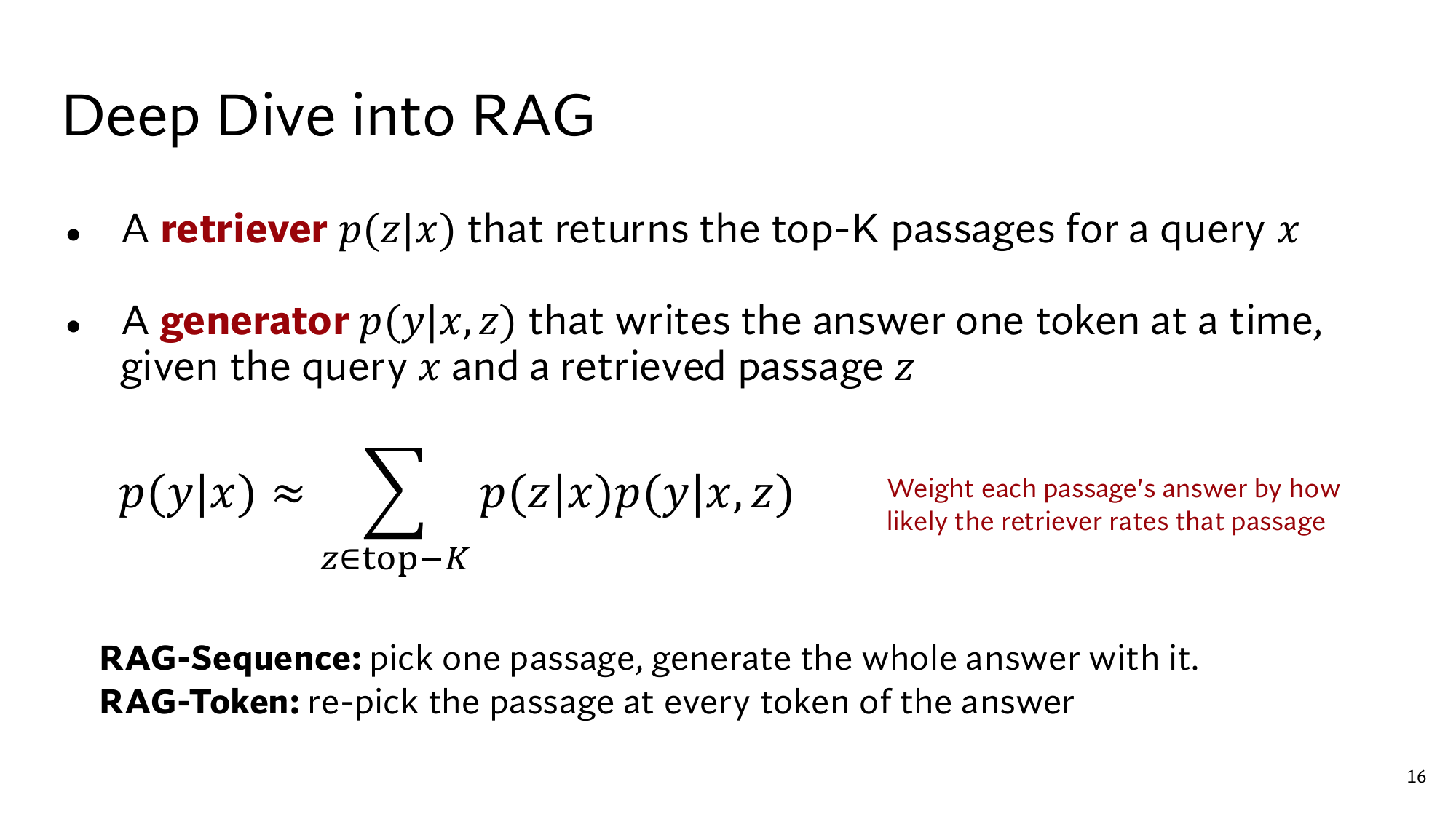
Stanford's slide: Deep Dive into RAG. At the top are the retriever p(z|x) and the p(y|x, z), the LLM that writes the answer. In the middle is this formula. The red note says to weight each passage's answer by how much the retriever trusts that passage. The RAG-Sequence and RAG-Token lines at the bottom come in lesson 5. Click the image to open it at full size.
Think first
Suppose the retriever trusts the wrong passage: the queue log gets score 0.0, and the forum post 1.0. The LLM's numbers stay at 0.9 and 0.1. What are the total probability of Thursday 9am and the loss now?
Show the answer
The weights flip: the queue log gets 0.269 and the forum post 0.731. Total probability = 0.269 × 0.9 + 0.731 × 0.1 = 0.242 + 0.073 = 0.315, and loss = −ln 0.315 = 1.155.
The LLM changed nothing, yet the probability fell from 0.685 to 0.315. Wrong weights drag the whole answer down, and in lesson 5 training fixes exactly this mistake.
What the dense version adds
The dense version contains this whole lesson, followed by 5 more steps that take you to the level of the Stanford slides:
Step 6: every symbol in the slide's formula, the generator's full product as the paper writes it, and the difference between p(A|B) and p(B|A). Also a check, with a third passage, of how close the ≈ is.
Step 7: the remaining rules of exp and ln, such as ln(a ÷ b) = ln a − ln b, and the fact that ln(a + b) does not split. Also log10 and −ln 0.
Step 8: softmax in full: negative scores, the effect of scale, the normalizer Z, column vectors and the transpose, and why MIPS is enough to find the top k.
Step 9: the slide's “negative marginal log-likelihood” word by word, the total loss over two examples, and the loss's rates for the retriever and the generator in numbers.
Step 10: Stanford's three slides, which you read yourself.
p(A|B) means “the chance of A, given B”. By the chain rule, the probability of a whole answer is the product of each token's conditional probability.
When you do not know which case is true, multiply each case's weight by the chance within that case, then add. That is marginalization, and it is the RAG formula of lesson 5.
Softmax turns scores into weights with exp and a division, and looks only at differences between scores. −ln p is the loss, and training uses the gradient to make it small.
New terms in this lesson
Conditional probability, p(A|B)
The probability of A when B is known. Read “|” as “given”. For example, p(full | Tuesday) = 16 ÷ 20 = 0.80.
Chain rule (for probabilities)
p(A and B) = p(A) × p(B|A). With many steps, multiply them all. For example, p(Tuesday) × p(full | Tuesday) = 0.5 × 0.8 = 0.40. The chain rule for rates in lesson 12 is a different rule.
∏ (capital pi)
Multiply everything over the range written below it. For example, for three tokens, 0.21 × 0.31 × 0.71 = 0.046.
Marginalization
Each case's weight times the probability within that case, added up over all cases. For example, 0.5 × 0.8 + 0.5 × 0.1 = 0.45.
≈
Approximately equal. The RAG formula adds up only the top-K passages, so the sum is only approximately equal.
exp and e
exp(s) = es, where e is about 2.718. Always above 0, and ea+1 = ea × e. For example, exp(1) = 2.718, exp(0) = 1, exp(−1) = 0.368.
Softmax
The exp of each score, divided by the sum of all the exps. It turns scores into probabilities. For example, 2.0, 1.0, 0.1 become 0.659, 0.242, 0.099.
∝
Is proportional to. At the end, divide everything by one number so that the total is 1. For example, exps 2.718 and 1 become 0.731 and 0.269.
d⊤q
A way of writing the dot product of vectors d and q. For example, the office hours page [0.9, 0.1] and the question [0.8, 0.2] give 0.74.
Natural log, ln
The power you raise e to in order to get x. ln(ex) = x, and ln(a × b) = ln a + ln b. For example, ln(0.1) = −2.303.
Loss
A number for how wrong the model is. Training makes it small. For example, if the right answer has probability 0.5, the loss is −ln 0.5 = 0.693.
Likelihood
The probability the model gave the correct data. For example, if it gave the right answer 0.12, the likelihood is 0.12.
Negative log-likelihood
−ln p(right answer). The most common loss. For example, at p = 0.12, −ln 0.12 = 2.120.
Gradient
The calculation of which way, and how much, to change each parameter so that the loss goes down. For example, in lesson 1 training moved the parameters in the direction that raised Thursday's probability from 0.10 to 0.12 and lowered the loss from 2.303 to 2.120.