How an LLM writes an answer, and where it gets stuck
An LLM is a model that reads text and writes the text that comes next, one token at a time. It picks each next token by looking at probabilities, and those probabilities come from its parameters and from the text you give it.
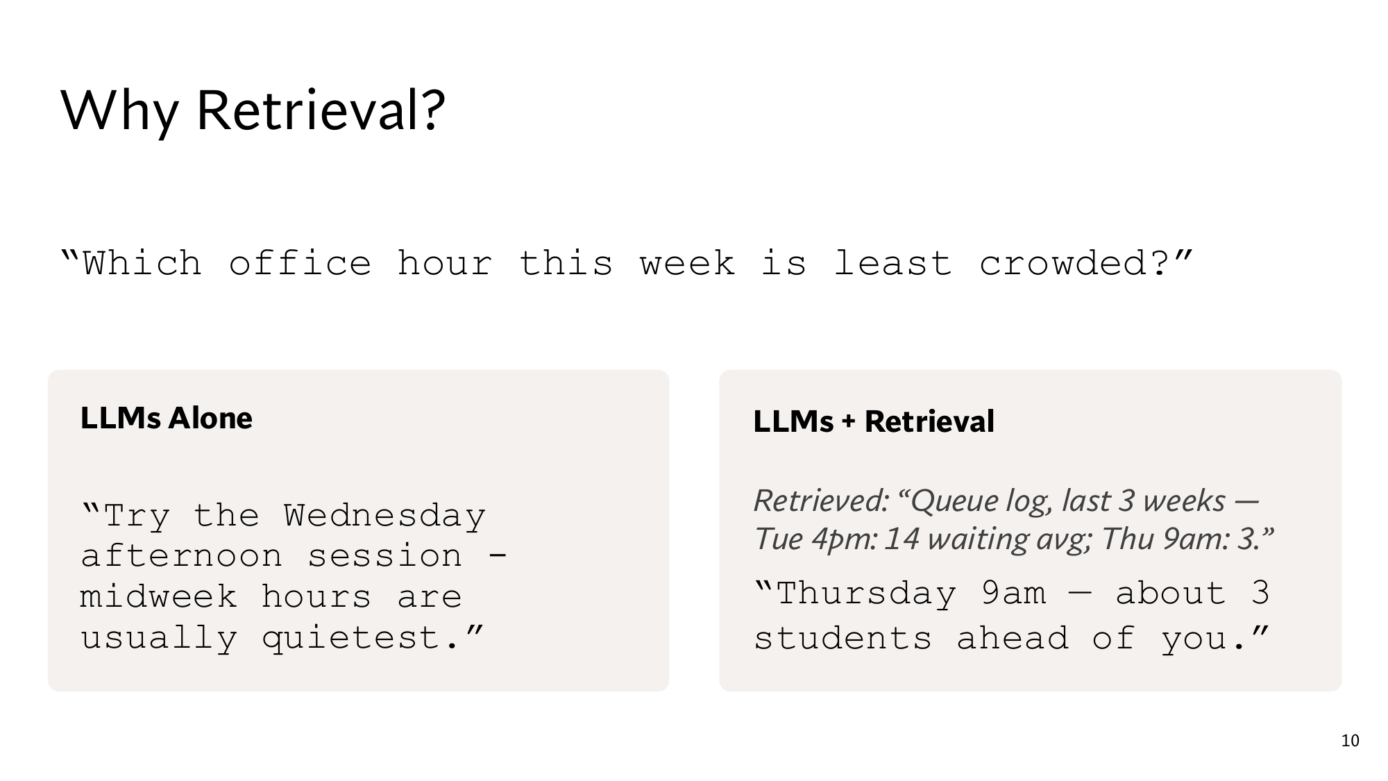
The lecture opens with a question: Which office hour this week is least crowded? The course's TAs, senior students who help with teaching, hold office hours twice a week: Tuesday 4pm and Thursday 9am. Office hours are fixed times when any student can drop in and ask questions. Ask an LLM on its own, and it answers with confidence: Try the Wednesday afternoon session - midweek hours are usually quietest.
The course keeps a queue log, a record of how many students were waiting in line at each office hour. Over the last 3 weeks, Tuesday 4pm averaged 14 students and Thursday 9am only 3. So the right answer is Thursday 9am, and there is no office hour on Wednesday at all. The LLM never saw this log, yet it did not hesitate for a moment. This lesson explains why.
The ladder for this lesson
The ladder has 9 steps. The first 5 are the same as in the easy version, and steps 6 to 9 take you to the level of the Stanford slides. Under each step you can see what you will be able to do after it.
What you need first: nothing, school maths is enough. From step 6 on, a few things are covered fully in lessons 2 to 5, and those places link to them. If you already know a step, skip to the next one. A word with a dotted underline and ▾ opens its definition when you click it.
1Tokens: the model reads pieces of text
A token is a small piece of text: sometimes a whole word, sometimes part of a word, sometimes a punctuation mark. An LLM reads text by splitting it into tokens, and it writes its answer in tokens too.
Tokens are needed because a computer can only calculate with numbers. The model has a fixed list of tokens, and each token in it has an ID number. This list is called the vocabulary, and the program that splits text into its tokens is called the tokenizer.
A common word is often a single token, while a rarer word breaks into a few pieces. For example, Office hours are crowded on Tuesday has 6 words but 7 tokens: my split
Office hours are crowded on Tuesday
Here crowded broke into two tokens, crowd and ed. In the same way, if the vocabulary has no entry for a misspelling like Wednesdayy, the tokenizer still splits it into Wednesday and y. The real split depends on each model's own tokenizer.
Since the model reads and writes only tokens, this lecture measures every length in tokens, not in words.
2Next-token prediction: one token per step
While writing an answer, an LLM gives every token a probability at each step, then picks one token and adds it to the text. Then it repeats the same thing on the new text. This loop is called next-token prediction, and the whole answer comes out of it.
A probability is a number between 0 and 1 that gives the chance of something happening: 0 means never, and 1 means certain. For example, if 5 of the last 20 lectures had a quiz, the probability of a quiz in the next one is 5 ÷ 20 = 0.25. The probability of no quiz is 15 ÷ 20 = 0.75, and the probabilities of all the options always add up to 1.
Now the model is given this text: The least crowded office hour this week is. Its probabilities for the next token might look like this: my numbers
Next token
Probability
" Wednesday"
0.34
" Thursday"
0.21
" Tuesday"
0.18
" Friday"
0.15
" Monday"
?
Sum
1.00
In reality, the thousands of other tokens also get very small probabilities. To keep the arithmetic small, assume there are only these 5 tokens.
Work out the Monday row
The five probabilities must add up to 1. What is Monday's probability?
Show the answer
The other four add up to 0.34 + 0.21 + 0.18 + 0.15 = 0.88. So Monday = 1 − 0.88 = 0.12.
Now suppose the model always takes the token with the highest probability. At the first step it takes Wednesday, and then it looks at the probabilities for the token after that. Press “Pick the highest” three times in the widget below. the later steps use my numbers too
Build an answer yourself
Click any token, or press “Pick the highest” three times.
After three steps the model writes what it wrote at the start of the lesson: Wednesday afternoon. At no step did it look at the queue log. Wednesday got 0.34 because people often write things like “midweek is quiet”. So a probability tells you which token is common after this text, not which one is true.
Real models often choose at random according to the probabilities. Then the 0.34 token comes up about 34% of the time, and the same question can get different answers.
Think first
In the widget you chose Thursday, morning and the full stop, the tokens at 0.21, 0.31 and 0.71. According to the queue log, Thursday 9am really is the least crowded. Did the model know the answer this time?
Show the answer
No. The answer came out right by luck. The model never saw the log, and it gave Thursday a lower probability than Wednesday.
3Parameters and training: where the model's knowledge lives
Parameters are the numbers inside a model. The input tokens are combined with these numbers by a fixed calculation, and that calculation produces the probability of every next token. Another name for parameters is weights, and there are a great many of them. The T5-11B model on Stanford's slides, for example, has about 11 billion parameters. from the paper
The values of these parameters are set by training. At first the parameters are random. Then the model reads a large amount of text, and at every position training checks what probability the model gave to the real next token. Then it nudges the parameters a little so that this probability goes up.
Here is one step. The training text contains the line Office hours are on Thursday. After reading Office hours are on, the model gives the next token Thursday a probability of 0.10. Training changes the parameters slightly, and now the same text gives Thursday 0.12. my example The total stays at 1, so all the other tokens together dropped from 0.90 to 0.88.
So whatever the model “knows” is spread across the values of its parameters, not stored in a separate file or database. Knowledge held this way is called parametric knowledge. Training stops on some date, and after that the parameters do not change. That date is called the knowledge cutoff.
The queue log is this course's own data, so it never went into any model's training. Its 14 and 3 are not in any parameter. This shows the two problems with parametric knowledge:
New facts do not get in. To add something from after the knowledge cutoff, or your private data, the model has to be trained again.
The model cannot name a source. The knowledge is mixed into billions of numbers, so the model cannot tell which document a fact came from.
4The prompt and the context window
The prompt is the text you give the model right now: the question, instructions, and any document that comes with them. At every step, next-token prediction looks at all the text so far, and that includes the prompt. So the prompt's text can change every probability, while the parameters stay the same.
Now put the queue log line in the prompt before the question, the line that says 14 for Tuesday 4pm and 3 for Thursday 9am.
Think first: The parameters are the same, and only the prompt changed. Will Thursday's 0.21 and Wednesday's 0.34 go up or down? Make a guess, then switch on the box below.
Change the prompt, watch the probabilities
The parameters stay the same. Only the prompt changes. my numbers
With the log added, Thursday's probability goes from 0.21 to 0.81, and Wednesday's from 0.34 to 0.05, while the parameters stay the same. Put information that is not in the parameters into the prompt, and the model uses it. The whole lecture is built on this.
The prompt has a limit too. The model can read only a fixed number of tokens at once, and this limit is called the context window. Both the prompt and the answer the model writes count toward it. For example, if the window is 8,000 tokens and the prompt is 7,500, only 500 tokens are left for the answer.
All of a course's documents together can be far larger than this window. So for every question you have to choose which pieces go into the prompt, and lesson 2 starts from that choice.
Think first
The context window is 8,000 tokens. The question and instructions take 300 tokens, and the answer needs 700. Each passage, a piece of a document, is 500 tokens. At most how many passages fit in the prompt?
Show the answer
That leaves 8,000 − 300 − 700 = 7,000 tokens for passages, and 7,000 ÷ 500 = 14 passages.
5Hallucination: a confident answer without data
A hallucination is an answer that reads well and sounds confident, but is wrong or does not rest on any source. The Wednesday afternoon answer is one, and its cause comes from putting the last three steps together.
The queue log was not in the parameters, because it never went into training (step 3). It was not in the prompt either (step 4). Even so, next-token prediction picks some token at every step, and the most common token was Wednesday (step 2).
Next-token prediction has no step that stops when the data is missing. So a wrong answer is written with the same confidence as a right one, and the reader cannot tell them apart.
Stanford's Why Retrieval slide. On the left is the LLM alone, which wrote Wednesday. On the right the prompt holds the queue log line, and the answer is Thursday 9am. Click the image to open it at full size.
The right half of the slide shows retrieval, which means finding the right text when the question arrives and putting it into the prompt. There the answer's 3 comes straight from the log line, so a reader can check it. Lesson 2 starts from here.
Think first
Which prompt gives the lowest chance of a hallucination? (a) Only the question. (b) The question and the queue log. (c) The question and an old 2024 forum post that says midweek afternoons are usually quiet.
Show the answer
(b). With (c), the model may trust the old post and write Wednesday again, so wrong text in the prompt also does harm. This point comes back in lesson 2.
From here: the Stanford level
The 5 steps above are the same as in the easy version. The 4 steps below take you to the level of the Stanford slides. They cover the slide's notation and the probability of a whole answer, then the numbers for models that answer from parameters alone, and then the papers' experiments. Finally you read the slides yourself. Every piece of maths is explained where it first appears.
6The slide's notation: p(y | x, z), θ, and the probability of a whole answer
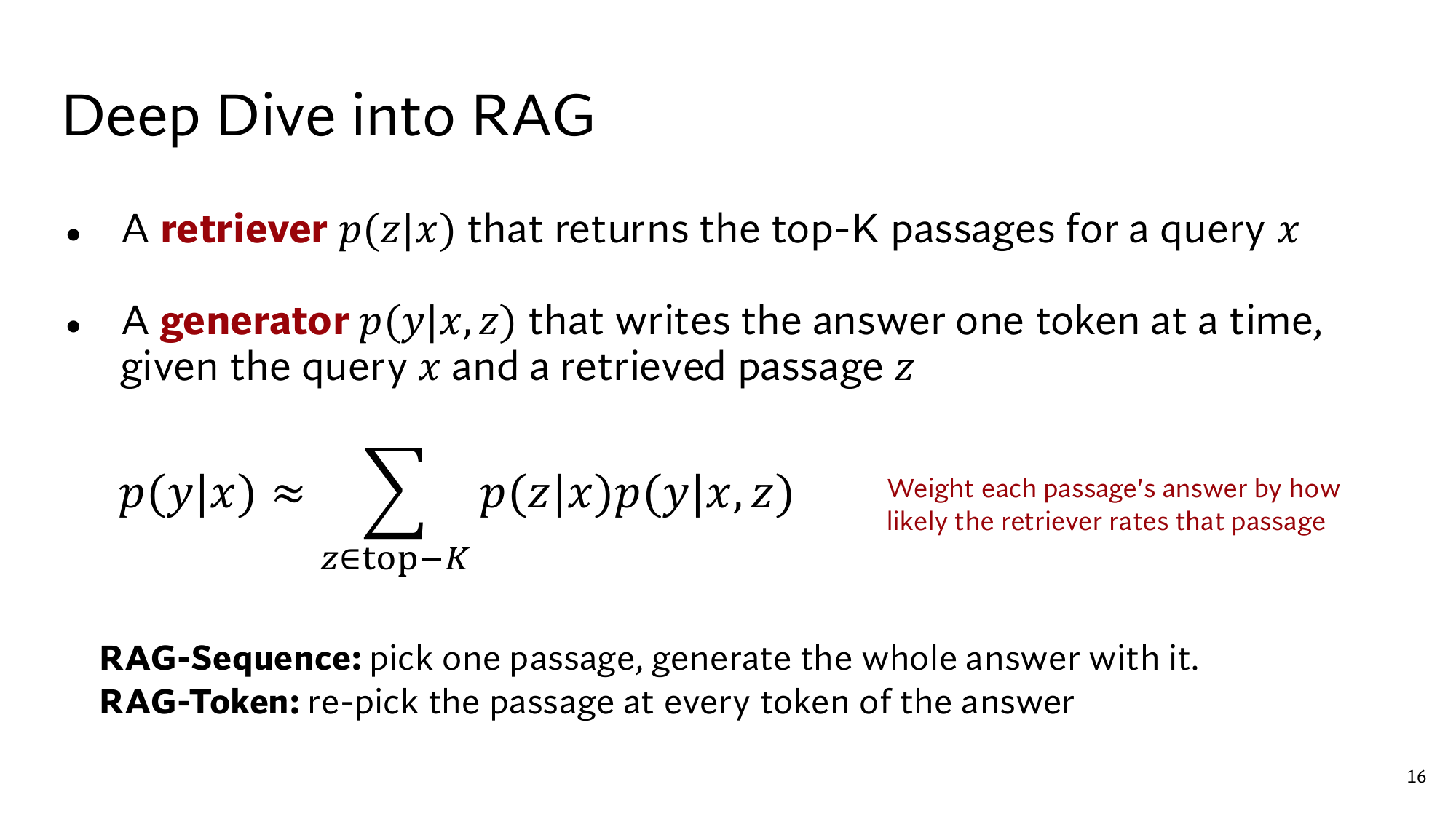
Stanford's slides call the LLM a generator and describe its job in one line:
A generator p(y|x, z) that writes the answer one token at a time, given the query x and a retrieved passage z.
This line is the next-token prediction of step 2, written in symbols. In this step you read every symbol in it with your own numbers.
The text after the “|”: p(y | x) and p(y | x, z)
Before the symbols, take two numbers from step 4. After the text The least crowded office hour this week is, Thursday got 0.21, and with the queue log line placed before it, 0.81. The token was the same, and only the text before it changed. The notation records exactly this difference:
Symbol
Meaning
In our example
x
The query, the text the model receives
The least crowded office hour this week is
z
A retrieved passage, a piece of a document placed in the prompt
The queue log line
y
The answer, or one of its tokens
Thursday
p(y | x)
The probability of y when only x is given
0.21
p(y | x, z)
The probability of y when both x and z are given
0.81
The vertical bar “|” is read “given”. After it comes the text the model already has, and the comma means “and”. Lesson 4 explains this fully under the name . For now it is enough that changing the text after the “|” changes the probability of the same token.
θ: the generator's parameters
On the slide the generator's full name is pθ. θ (theta) is the name for the generator's parameters, all the numbers from step 3. Writing θ underneath says that these probabilities come from those parameters. The retriever's parameters are called η (eta), and they come in lesson 5.
The training step from step 3 looks like this in the notation: pθ(Thursday | Office hours are on) was 0.10, and after θ changed slightly it became 0.12. There the text stayed the same and θ changed. In step 4 it was the other way round: θ stayed the same, and the text after the “|” changed.
One token at a time: the probability of a whole answer
The generator writes the answer one token at a time, so the probability of the whole answer is built from the probability of each token. Counting shows this most clearly. Suppose the model writes the same answer 1,000 times, choosing at random each time with the widget's probabilities: my numbers
At the first step, Wednesday comes up about 1,000 × 0.34 = 340 times.
In 46% of those 340, the next token is afternoon: 340 × 0.46 = 156.4, so about 156 times.
In 71% of those, a full stop follows: 156.4 × 0.71 = 111.0, so about 111 times.
111 times out of 1,000 means the whole answer Wednesday afternoon. has probability 0.111. That is the product of the three probabilities: 0.34 × 0.46 × 0.71 = 0.111. Each step keeps a share of the cases left by the step before, which is why the probabilities multiply. The formula writes the same product like this:
Here y1 = Wednesday (0.34), y2 = afternoon (0.46) and y3 = the full stop (0.71). After the “|” of each token come the question and all the tokens before it, because next-token prediction looks at all the text so far at every step. The RAG paper writes each token's probability as pθ(yi | x, z, y1:i−1), where y1:i−1 means tokens 1 to i − 1. from the paper
Think first
Take the widget's other answer, Thursday morning., whose tokens have probabilities 0.21, 0.31 and 0.71. What is the probability of this whole answer, and how many times more often does Wednesday afternoon. come up?
Show the answer
0.21 × 0.31 = 0.0651, and 0.0651 × 0.71 = 0.046, so about 46 times in 1,000. Wednesday afternoon comes up 0.111 ÷ 0.046 = 2.4 times as often.
The same product shows one more thing. Every probability is below 1, so every extra token lowers the probability of the whole answer. Even this widget's most common answer sits at only 0.111, which means that about 889 times in 1,000 the model writes something else.
Greedy decoding and sampling
There are two common ways to pick a token, and both appeared in step 2. Taking the highest-probability token at every step is called greedy decoding. The widget's “Pick the highest” does this, and its answer is always Wednesday afternoon. Choosing at random according to the probabilities is called sampling, and the 1,000-run count above was sampling.
With sampling, the first token can change from run to run. Run it 100 times and you get Wednesday about 34 times, Thursday 21, Tuesday 18, Friday 15 and Monday 12. So sampling sometimes writes the right Thursday too, but only by luck, as in the question in step 2.
For question answering, papers often use greedy decoding. The T5 paper in step 7 picks the most likely token at each step, and the RAG paper also uses greedy decoding for question answering. from the paper
7Closed-book QA: how many answers come from parameters alone
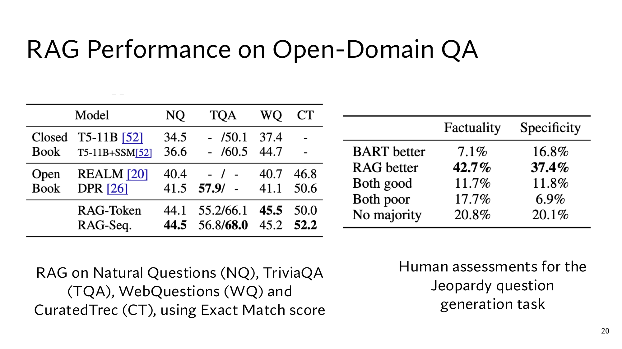
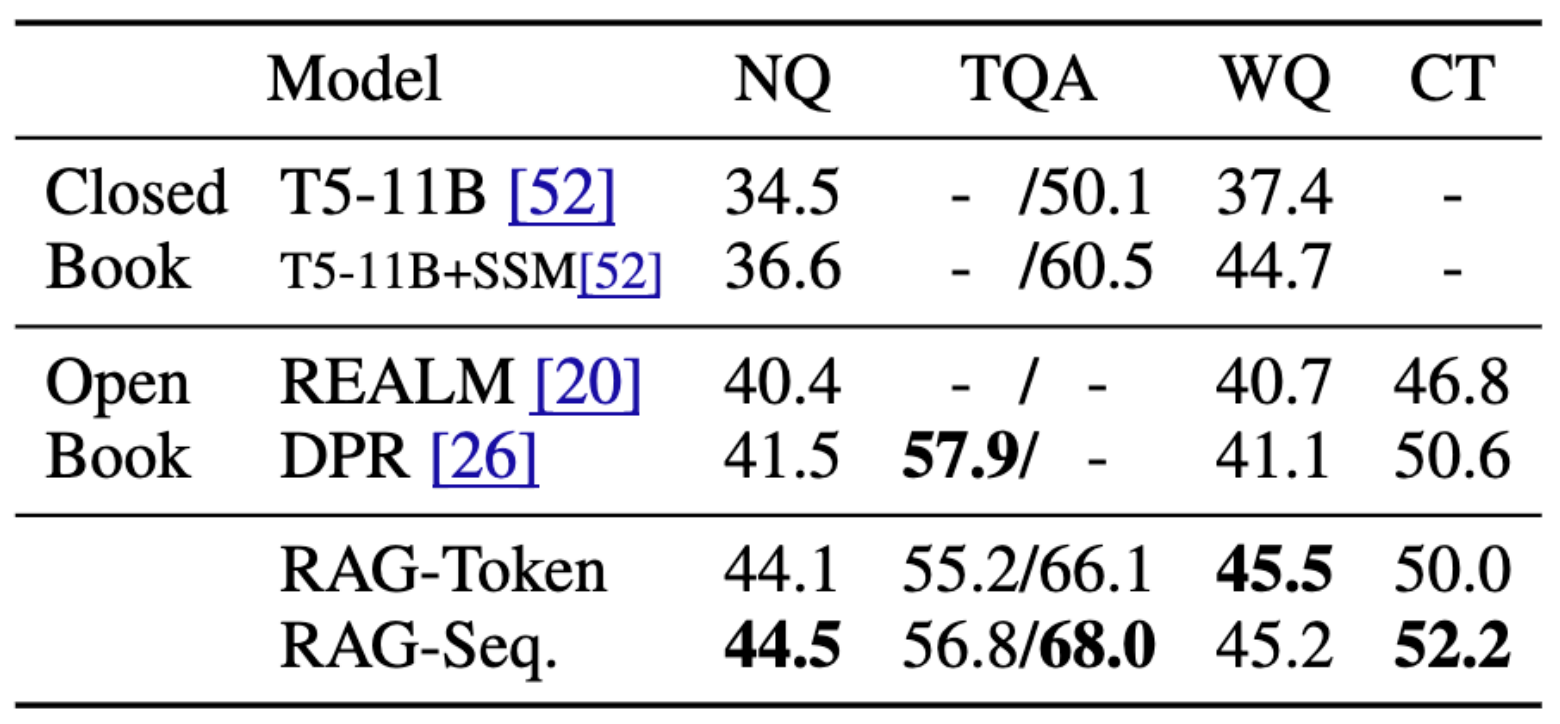
In closed-book question answering the model gets only the question and no document, so it writes the answer from its parameters alone. That is exactly what the LLM on its own did at the start of the lesson. In the open-book setting the system first searches documents and then writes the answer. Stanford's RAG Performance slide compares models.
The slide's closed-book rows come from a 2020 paper by Roberts and colleagues. They taught Google's T5, a model that reads text and writes text, to answer questions given only the question, with no documents at all. from the paper From here on this paper is called the T5 paper.
Exact Match: did the answer match word for word
The numbers in these tables are scores: the percentage of questions where the model's answer matches the correct answer exactly. Before matching, both are lowercased, and a, an, the, punctuation and extra spaces are removed. from the paper For example, if the correct answer is Thursday 9am, then thursday 9am. matches. But Thursday 9 am does not, because it has a space between 9 and am.
The four columns of the slide's table are four datasets. NQ is Natural Questions, real questions people typed into Google search. TQA is TriviaQA, questions from quiz websites. WQ is WebQuestions and CT is CuratedTrec, two smaller question-answer datasets. from the paper
What changes when the parameters grow
T5 comes in four sizes, and the paper trained all four in the same way to answer questions. Below are the numbers on TriviaQA's Wikipedia test set: from the paper
Model
Parameters
TriviaQA (%)
T5-Base
220 million
29.1
T5-Large
770 million
35.9
T5-3B
3 billion
43.4
T5-11B
11 billion
50.1
T5-11B + SSM
11 billion
60.5
From Base to 11B the parameters grow 11,000 ÷ 220 = 50 times, and the score rises from 29.1 to 50.1, a gain of 21.0 points. Each larger size answers more questions exactly right, so a bigger model holds more knowledge in its parameters. This TriviaQA column is used because its 50.1 and 60.5 are the same numbers as on Stanford's slide. For NQ, the current version of this paper gives T5-11B 32.6 while the slide says 34.5, so for NQ use the slide's number.
The SSM in the last row, salient span masking, is an extra round of training. In it the model reads Wikipedia sentences with blanks where names and dates were, and has to fill in the blanks. T5 ran this round for 100,000 extra steps, and the TriviaQA score went from 50.1 to 60.5. from the paper This round is part of , the large training on general text that comes before the model is taught to answer questions.
Fewer parameters, with documents
Now look at the NQ column of the slide's table. In the closed-book rows, T5-11B is at 34.5, and 36.6 with SSM. In the open-book rows, RAG-Seq. is at 44.5. Out of 1,000 questions, that is 345 against 445 exactly right answers, so the system with documents gets 100 more questions right.
RAG's generator is a model called , with about 400 million parameters, and the whole of RAG has about 626 million. T5-11B has 11 billion, which is 11,000 ÷ 626 = 17.6 times as many. The RAG paper also notes that T5-Large, with 770 million parameters, scores 28.9 on NQ. from the paper
So with documents at hand, a system with 17.6 times fewer parameters is still 10 points ahead on NQ. The RAG paper draws the same conclusion: a system that combines parameters with documents needs far fewer parameters to answer questions well. The gain comes from step 4, because the text with the answer reaches the prompt.
8The papers' experiments: measuring hallucination and the knowledge cutoff
Steps 3 and 5 named three weaknesses of parametric knowledge: new facts do not get in, there is no source, and an answer comes out even without the data. The RAG paper opens with the same three. Such models cannot easily expand or revise their memory, cannot show why they predicted something, and can hallucinate. from the paper The three experiments in this step put numbers on them.
150 answers Exact Match called wrong, checked by hand
The T5 paper checked by hand 150 answers on NQ that Exact Match had marked wrong. They fell into four groups: from the paper
Group
Answers
Share
Really wrongWhat does the Ghost of Christmas Present sprinkle from his torch? Correct: warmth. T5: confetti.
93
62.0%
Different wordingFor example, April 15 and April 15th.
20
13.3%
Incomplete list of correct answersWhere does the US launch space shuttles from? The list has only florida. T5: kennedy lc39b.
20
13.3%
The answer depends on when it is askedWho is the secretary of state for Northern Ireland?
17
11.3%
The arithmetic: 93 + 20 + 20 + 17 = 150, and 93 ÷ 150 = 0.620, 20 ÷ 150 = 0.133, 17 ÷ 150 = 0.113. So Exact Match underrates a closed-book model, but 62% of these answers were still really wrong. The confetti answer reads just as well as a correct one, and that is a hallucination. The last row ties to the knowledge cutoff, because its answer changes over time while the parameters stay fixed at training time.
At the end of the paper the authors themselves name three points. The model spreads knowledge across its parameters in a way nobody can explain. When it is unsure, it makes up realistic-looking answers. And after training there is no way to add or remove a specific fact. from the paper
Jeopardy questions: people judged factuality
In the RAG paper, people checked hallucination directly. Jeopardy is a quiz format where the answer comes first, and you write a question that has it as its answer. For the answer The World Cup, for example: In 1986 Mexico scored as the first country to host this international sports competition twice.from the paper
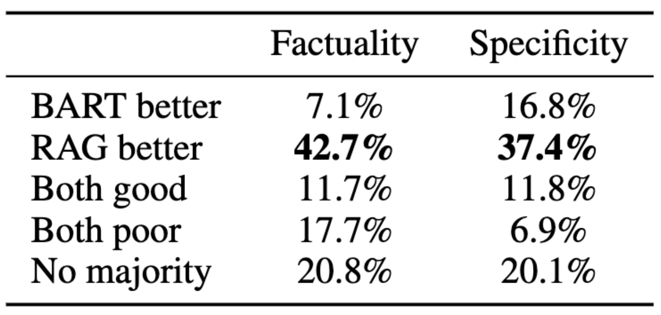
Two models wrote such questions. BART is a generator on its own, writing only from its parameters. RAG has the same BART, but its prompt also holds Wikipedia passages. People read 452 pairs and, for each pair, chose which question was more factual, meaning whose statement can be backed up by a trusted source.
People's verdict
Factuality
RAG better
42.7%
BART better
7.1%
Both good
11.7%
Both poor
17.7%
No majority
20.8%
Sum
100.0%
Of 452 pairs, 42.7% is about 193 pairs and 7.1% about 32. my arithmeticSo RAG's question was judged more factual 42.7 ÷ 7.1 = 6.0 times as often.
In the paper's table of examples, BART's wrong answers also read perfectly well. In Jeopardy, for Washington, BART wrote This state has the largest number of counties in the U.S., which the paper marks as wrong. For the same answer RAG wrote It’s the only U.S. state named for a U.S. president. from the paper
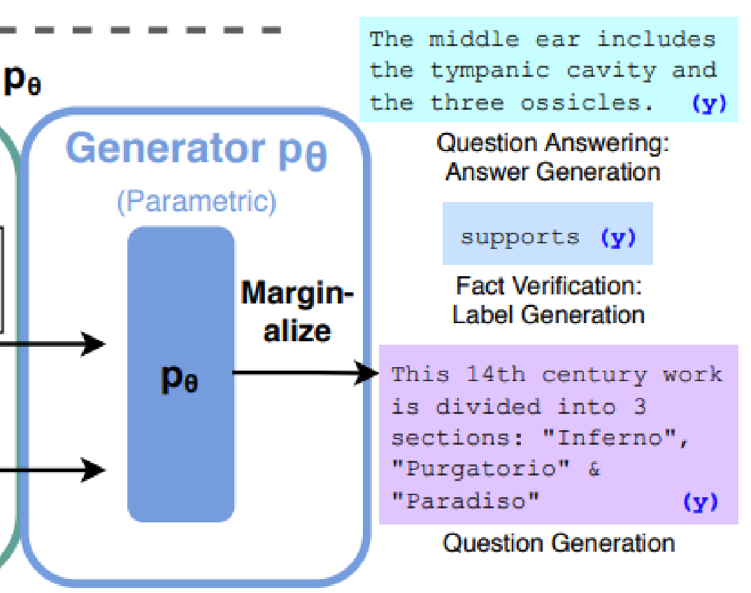
In another task the model had to write a one-sentence answer to define middle ear. There BART wrote that the middle ear is the part of the ear between the middle ear and the nose, which is wrong. RAG wrote The middle ear includes the tympanic cavity and the three ossicles.from the paper
New knowledge by swapping the documents: index hot-swapping
The first problem in step 3 was that adding a new fact needs training again. RAG keeps its documents in an , a list of passages organised so the retriever can search it fast. The RAG paper built two indexes from Wikipedia, one from December 2016 and one from December 2018. from the paper
The paper then listed 82 world leaders who changed between those two dates, and asked the model questions like Who is the President of Peru?. The model's parameters were the same in all four cases, and only the index changed: from the paper
Index ↓ / leaders of which year →
2016
2018
December 2016 index
70%
4%
December 2018 index
12%
68%
With the index from the right year, 68% to 70% of the answers are correct, and with the wrong year only 4% to 12%. So swapping the documents changed what the model knows, and it took no training. Replacing the index like this is called index hot-swapping. Lesson 2 calls this route : knowledge kept outside the parameters, in documents.
Think first
The course moved the Thursday office hour from 9am to 10am. What has to change to get this right in a system with an LLM alone, and in a system with documents?
Show the answer
For the LLM alone, the parameters have to change, which means training again. In the system with documents, changing the office hours passage is enough, because on the next question the retriever brings the new passage into the prompt. The paper's 2016 and 2018 experiment shows exactly this.
9Now read Stanford's slides yourself
Below are the four Stanford slides this lesson rests on, unchanged. Under each slide are a few questions. Think of the answer first, then open it. If a symbol stops you, go back to the step named in the answer. If a slide looks small on a phone, click the image to open it at full size.
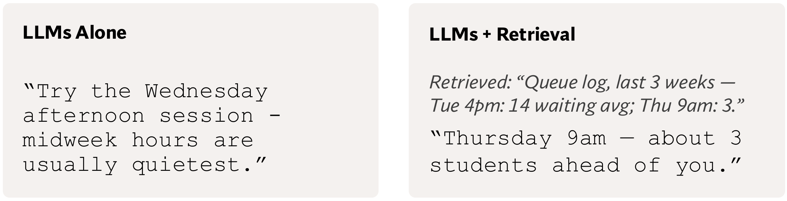
Stanford's Why Retrieval slide, and below it the two boxes, enlarged.
Read the Why Retrieval slide
Why did the LLM in the left box write Wednesday afternoon, when there is no office hour that day?
Show the answer
The queue log was neither in the parameters nor in the prompt. Next-token prediction still picks some token at every step, and the most common one was Wednesday. The probability said what is common, not what is true. (Steps 2, 3 and 5)
How did the Retrieved line in the right box reach the model, and what changed for the model?
Show the answer
The line is in the prompt. The parameters are the same, and only the text after the “|” changed, so p(Thursday | x) = 0.21 became p(Thursday | x, z) = 0.81. (Steps 4 and 6)
Where does the 3 in about 3 students ahead of you come from, and why is this not a hallucination?
Show the answer
The log line has 3 next to Thu 9am, and the answer took that number. The answer rests on a source that the reader can check. (Steps 4 and 5)
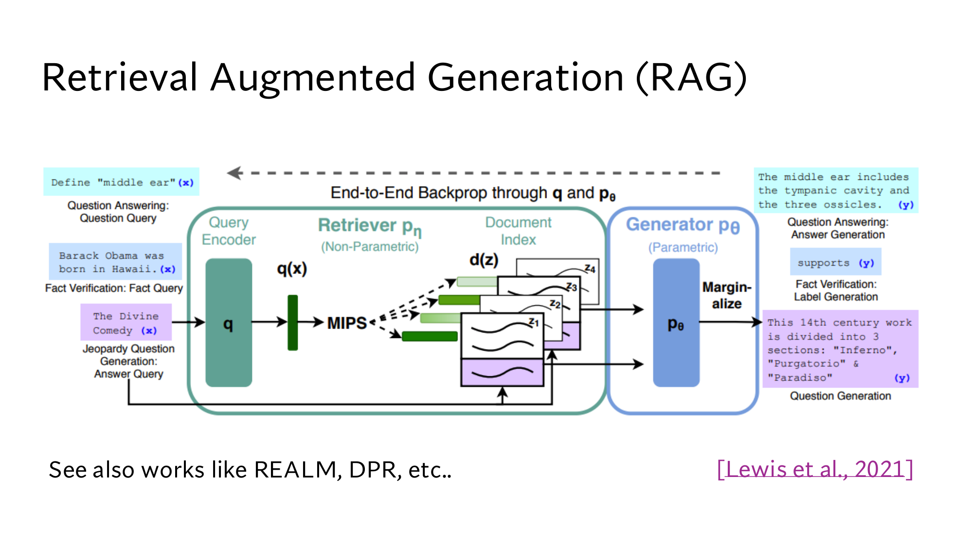
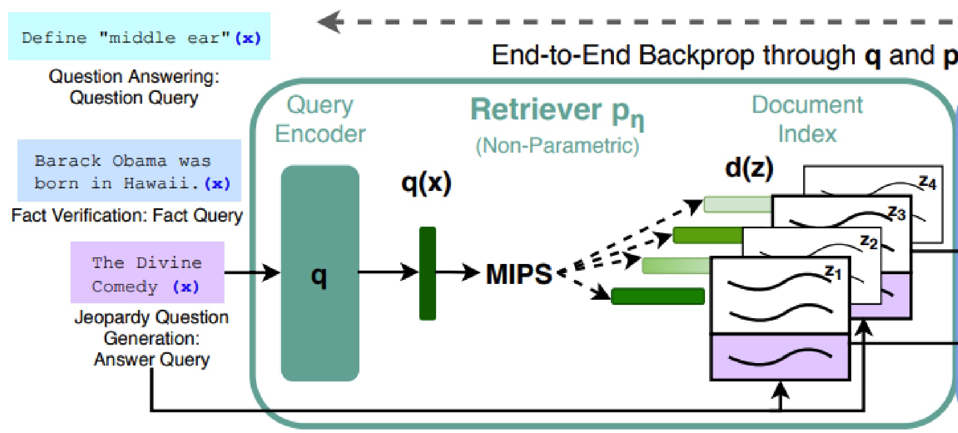
Stanford's slide: Retrieval Augmented Generation (RAG), and below it the generator part and the retriever part, enlarged.
Read the RAG slide
Why does it say (Parametric) under the generator and (Non-Parametric) under the retriever?
Show the answer
The generator's knowledge is in its parameters θ, which is parametric knowledge. Behind the retriever is the Document Index, where the passages' text lives outside the parameters and can be changed without training. (Steps 3, 6 and 8)
Who wrote the top y on the right, The middle ear includes the tympanic cavity and the three ossicles.? What did BART on its own write for the same question?
Show the answer
This is the answer of RAG, the model with documents. BART on its own wrote that the middle ear is the part of the ear between the middle ear and the nose, which is wrong. (Step 8)
What do the other parts of the slide do?
Show the answer
On the left are three kinds of input x: a question, a fact to check, and a Jeopardy answer. The Query Encoder q turns the question into a vector q(x), and the Document Index holds a vector d(z) for every passage (lesson 3). MIPS, maximum inner product search, finds the passages z1 to z4 with the largest dot products (lesson 2 and lesson 5).
Marginalize combines the answers written with several passages (lesson 4). The dashed arrow at the top is training, which changes q and pθ together (lesson 5).
Stanford's slide: Deep Dive into RAG, and below it the formula, enlarged.
Read the Deep Dive slide
Read p(y|x, z) in the generator line with our example: what are x, z and y?
Show the answer
x is the text the model receives, z is the queue log line, and y is Thursday. p(Thursday | x, z) = 0.81, while without z, p(Thursday | x) = 0.21. (Step 6)
Writes the answer one token at a time: how do you get p(y|x) for the three-token answer Wednesday afternoon.?
Show the answer
Take each token's probability, given the text before it, and multiply them all: 0.34 × 0.46 × 0.71 = 0.111. (Step 6)
What are the ∑, p(z|x) and ≈ doing in the formula?
Show the answer
The retriever brings several passages, and p(z|x) is how much it trusts each one. With each passage the generator gives the answer a different probability, and the ∑ adds these up weighted by that trust, as the red note says. The sum runs only over the top-K passages, the K highest-scoring ones, so it is ≈ rather than =.
Lesson 4 works this sum by hand, and the two lines at the bottom, RAG-Sequence and RAG-Token, come in lesson 5.
Stanford's slide: RAG Performance on Open-Domain QA, and below it both tables, enlarged.
Read the RAG Performance slide
What knowledge do the two Closed Book rows answer from, and how far behind RAG-Seq. are they on NQ?
Show the answer
From parameters alone. T5-11B is 44.5 − 34.5 = 10.0 points behind, and even with SSM it is 44.5 − 36.6 = 7.9 behind. REALM and DPR are open-book systems that pick the answer out of passages (lesson 5 and lesson 12). (Step 7)
What is the SSM in T5-11B+SSM, and what does “- /50.1” in the TQA column mean?
Show the answer
SSM is an extra round of training in which the model fills in blanks where names and dates were. TQA has two test sets: the usual open-domain one on the left and the Wikipedia one on the right. T5 was measured only on the Wikipedia one, so the left slot shows “-”. (Step 7)
According to the RAG paper the Wikipedia questions are easier, which is why RAG-Seq. also scores 68.0 there instead of 56.8. from the paper
What do the 42.7% and 7.1% under Factuality in the right table say? What does that column add up to?
Show the answer
Across 452 pairs, people judged RAG's question more factual 42.7% of the time, and BART's on its own only 7.1% of the time. The column adds up to 7.1 + 42.7 + 11.7 + 17.7 + 20.8 = 100.0. (Step 8)
Specificity means how closely a question is tied to its own answer. That column adds up to 93.0, not 100, and the paper does not say why.
3 points from this lesson
An LLM writes one token at a time. The probability of a whole answer is the product of its tokens' probabilities, for example 0.34 × 0.46 × 0.71 = 0.111.
Knowledge comes from two places: the parameters and the prompt. T5-11B, with parameters alone, scores 34.5 on NQ, while RAG with documents scores 44.5 with 17.6 times fewer parameters.
A probability says what is common, not what is true. People judged RAG's questions more factual 6 times as often as BART's alone, and swapping the index brought in new knowledge without training.
New terms in this lesson
LLM
Large language model: a model that reads text and writes what comes next, one token at a time. For example, the model that wrote Wednesday afternoon.
Token
A small piece of text: a word, part of a word, or punctuation. The model reads and writes these. For example, crowded is two tokens, crowd and ed.
Vocabulary
The model's fixed list of tokens, each with an ID number. For example, it contains Wednesday but not Wednesdayy.
Tokenizer
The program that splits text into the vocabulary's tokens. For example, it splits Wednesdayy into Wednesday and y.
Probability
A number between 0 and 1 that gives the chance of something. The options always add up to 1. For example, a quiz in 5 of 20 lectures gives 5 ÷ 20 = 0.25.
Next-token prediction
Looking at the text so far, giving every token a probability, picking one, adding it, and repeating. For example, Wednesday, then afternoon, then a full stop.
Parameters (weights)
The numbers inside a model that produce the probability of every next token. For example, T5-11B has about 11 billion parameters.
Training
Changing the parameters little by little so that the real next token in the text gets a higher probability. For example, Thursday after Office hours are on goes from 0.10 to 0.12.
Parametric knowledge
Knowledge spread across the parameters. The model cannot name its source, and a new fact needs training again.
Knowledge cutoff
The date on which training stopped. Later events, and your private data, are not in the model. For example, with a March 2026 cutoff, an October 2026 announcement is not in the model.
Prompt
The text you give the model right now: the question, instructions, and accompanying documents. For example, the queue log line that lifted Thursday from 0.21 to 0.81.
Context window
The most tokens a model can read at once. Both the prompt and the answer count. For example, an 8,000-token window with a 7,500-token prompt leaves 500 for the answer.
Hallucination
A confident answer that is wrong or has no source. For example, Wednesday afternoon, written without seeing the log.
Greedy decoding and sampling
Greedy decoding takes the highest-probability token at every step, and sampling chooses at random according to the probabilities. For example, greedy always writes Wednesday afternoon, while sampling starts with Thursday about 21 times in 100.
Salient span masking (SSM)
An extra round of pretraining in which the model fills in blanked-out names and dates in Wikipedia sentences. For example, it lifted T5-11B's TriviaQA score from 50.1 to 60.5.
BART
A model that reads text and writes text, with about 400 million parameters. It is RAG's generator. For example, in the Jeopardy test BART on its own was judged more factual in only 7.1% of pairs.
Index hot-swapping
Replacing the document index without touching the parameters, so that the model's knowledge changes. For example, the 2018 index answered 68% of questions about 2018 leaders correctly, and the 2016 index only 4%.