RAG is a model made of two models. The retriever brings passages for a question and gives each one a weight, and the generator writes the answer with each passage. Both are trained together with one loss, and that training needs only question-answer pairs. RAG stands for Retrieval-Augmented Generation, a model published by Lewis and colleagues in 2020.
The need for it showed up in the last question of lesson 4. There the retriever gave the old forum post a weight of 0.731 and the queue log only 0.269. The generator's numbers stayed the same, yet the probability of the right answer, Thursday 9am, fell from 0.685 to 0.315. The mistake is the retriever's, but the training data holds only questions and answers. Nothing in it says the answer came from the queue log, and RAG teaches the retriever anyway.
The ladder for this lesson
The ladder has 10 steps. The first 5 are the same as in the easy version, and steps 6 to 10 take you to the level of the Stanford slides. Under each step you can see what you will be able to do after it.
What you need first: Lesson 2 (retriever, top-K), Lesson 3 (vector, dot product, encoder, index) and Lesson 4 (marginalization, softmax, ∏, loss). From step 6 on, step 9 of lesson 4's dense version (rates, the negative marginal log-likelihood) also helps. If you already know a step, skip to the next one. A word with a dotted underline and ▾ opens its definition when you click it.
1RAG's two models: retriever and generator
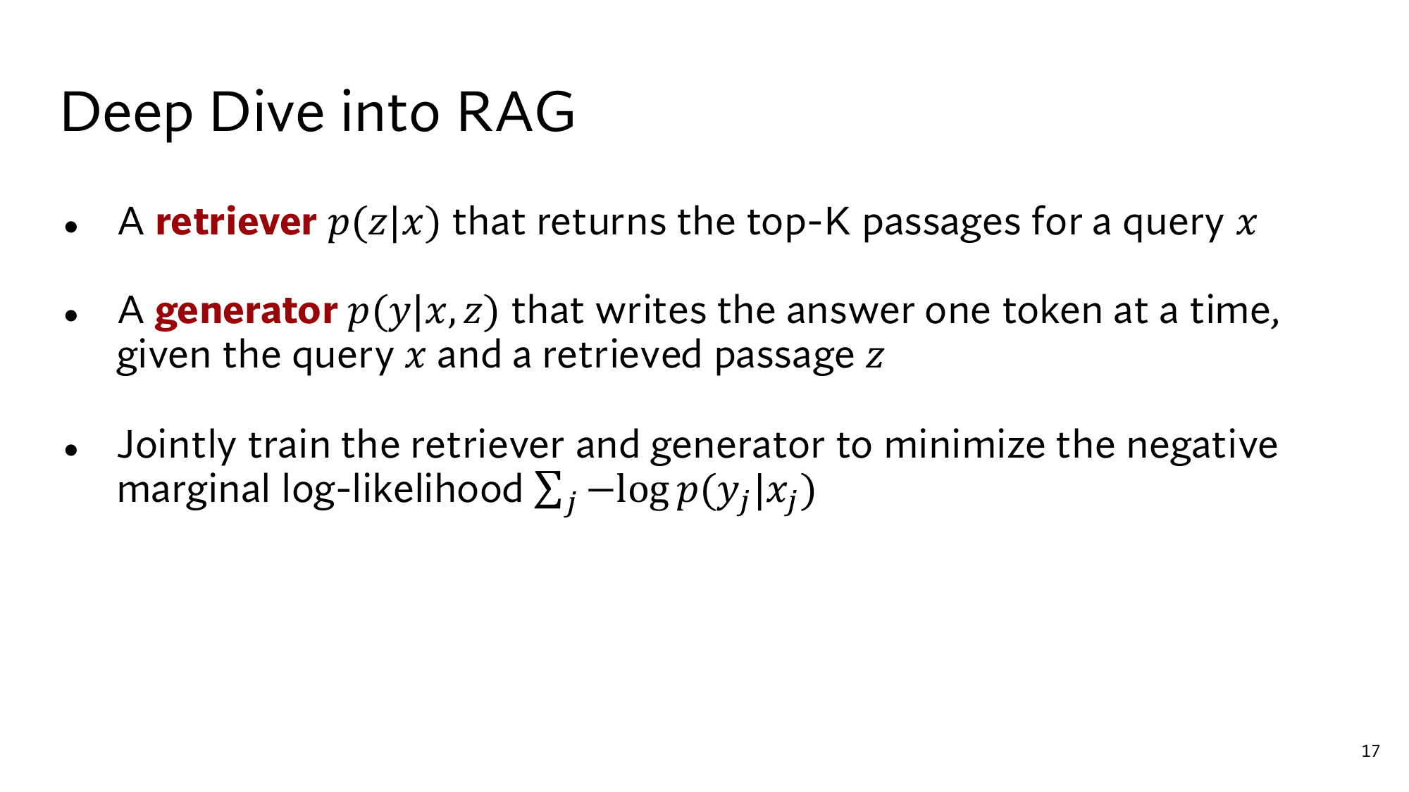
RAG contains two models. The retriever pη(z|x) gives every passage z a weight, and the generator pθ(y|x, z) reads the question x and one passage and writes the answer y. These are the same two probabilities that appeared in the formula of lesson 4. The small η (eta) and θ (theta) written underneath name the two models' , the numbers that training changes.
The retriever: DPR
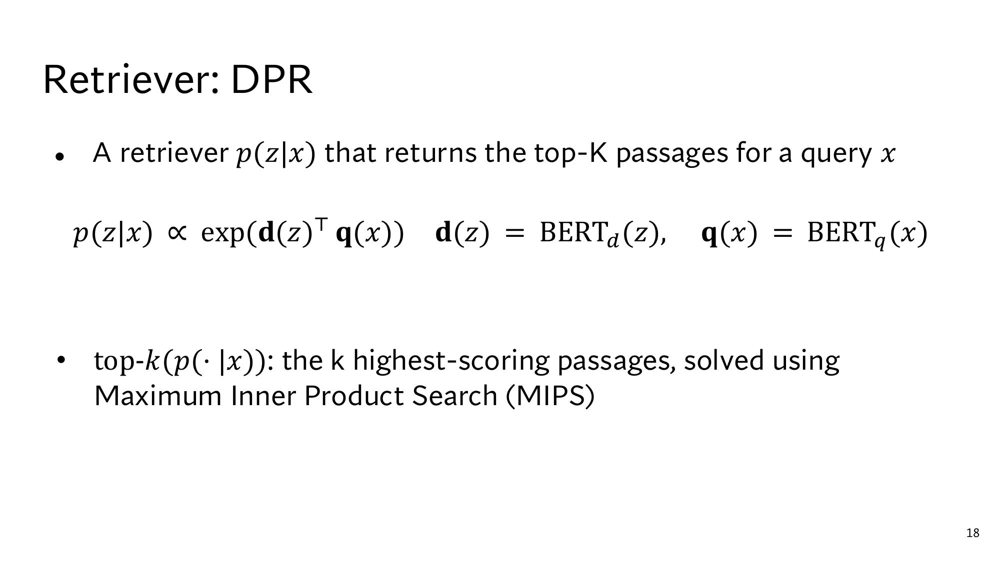
RAG's retriever is a model called DPR, whose own training comes in lesson 12. It has two , both built from BERT, an encoder model Google released in 2018. The query encoder makes the question's vector q(x), and the passage encoder makes a vector d(z) for every passage z.
A passage's score is the of these two vectors, written d(z)⊤q(x). Then turns the scores into weights that add up to 1. In lesson 4, scores 1.0 and 0.0 became weights 0.731 and 0.269. Stanford's slide writes the same thing like this:
pη(z|x) ∝ exp(d(z)⊤q(x))
Here means: take each passage's exp, then divide them all by one and the same number so that they add up to 1.
There are a great many passages. In the paper, Wikipedia is cut into about 21 million passages of 100 words each. from the paper Their vectors are built once, before any question arrives, and kept in an . When a question arrives, only the query encoder runs, and then a search pulls out the passages with the K largest dot products. This search is called MIPS, maximum inner product search, because inner product is another name for the dot product.
The generator: BART
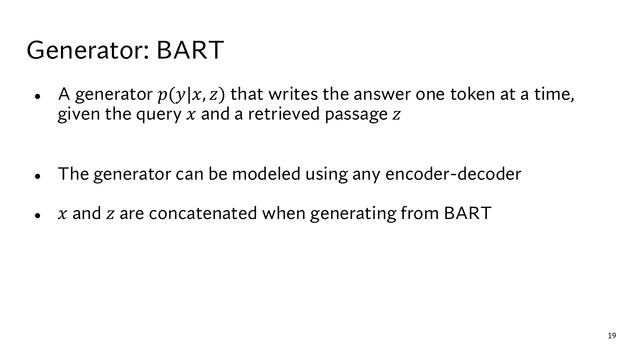
The generator reads the question and one passage and writes the answer, one token at a time, like the LLM in lesson 1. RAG's generator is , an encoder-decoder model. Its encoder reads the input text and turns it into vectors, and its decoder looks at those vectors while it writes the answer token by token.
BART reads a single text, so the question and the passage are joined end to end into one text. Joining two texts like this is called concatenating them. With the queue log, the input and the output look like this: my example
Input: question: Which office hour is least crowded? passage: Queue log, last 3 weeks: Tuesday 4pm office hour averaged 14 students waiting; Thursday 9am office hour averaged 3. Output: Thursday 9am
Question xWhich office hour is least crowded?
Query encoder q(x)The question's vector
MIPSDot product with every d(z) in the index, top-K
z1 … zKA weight for each, from softmax
Generator pθRuns once per z
MarginalizeAdd up to get p(y|x)
RAG's whole path for one question. The first four boxes are the retriever, and the last two are the generator. The Marginalize box comes in step 2.
This design has a cost. The generator runs separately with each passage, so with K = 5 it runs 5 times for one question.
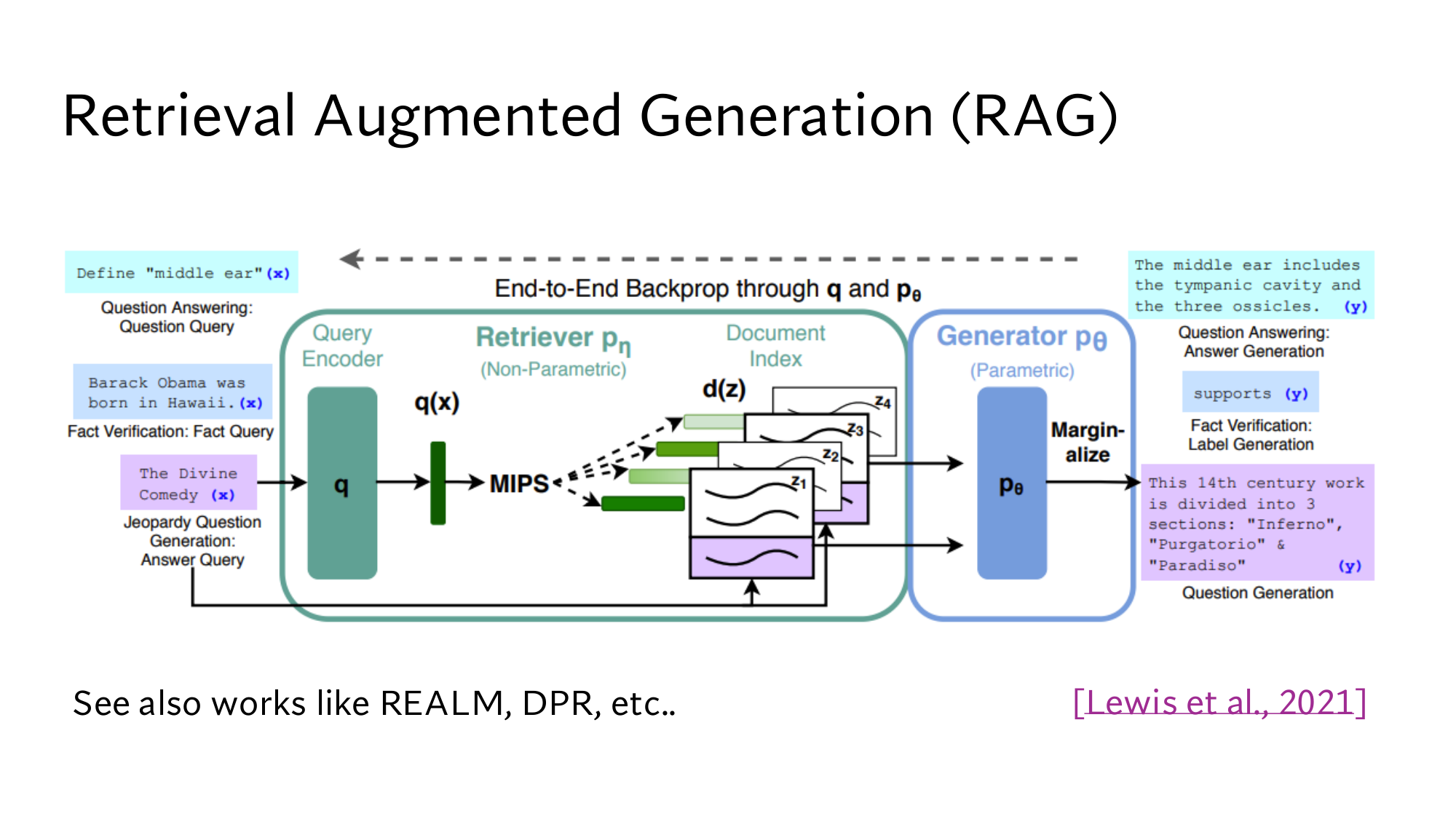
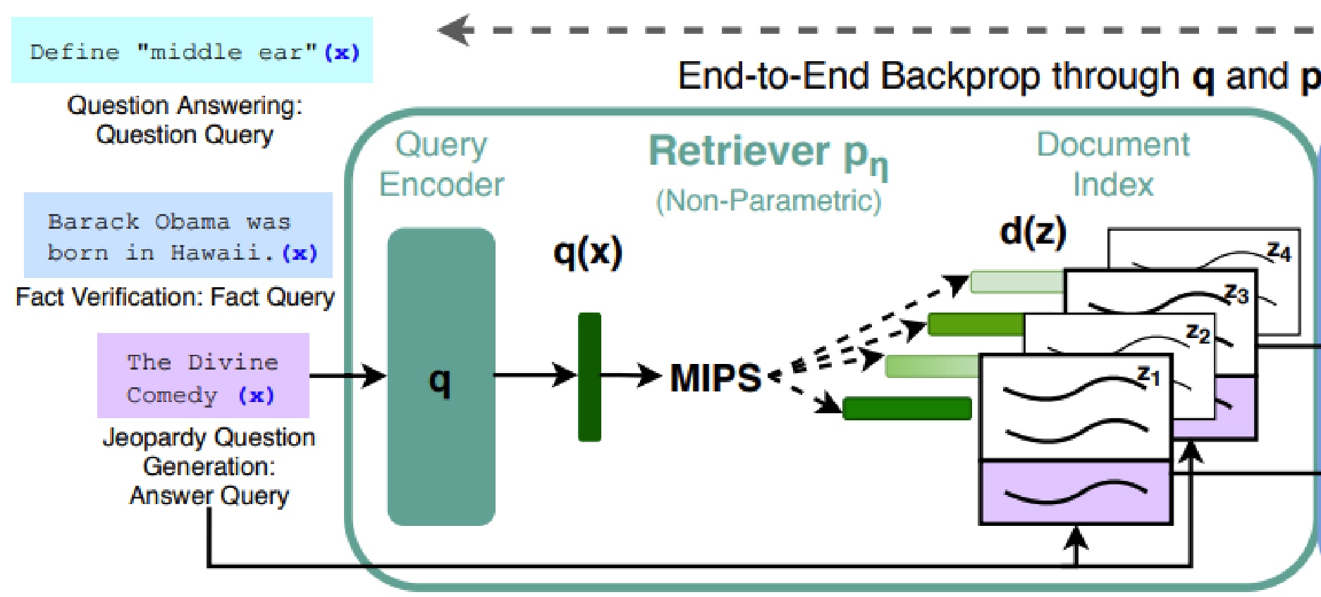
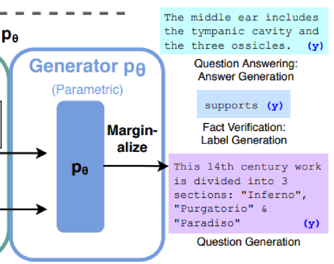
Stanford's slide: the RAG design. The green box is the retriever pη, holding the query encoder q, MIPS and the document index d(z). The blue box is the generator pθ. The dashed arrow at the top is training, which comes in step 4. Click the image to open it at full size.
2Marginalization: no passage label needed
RAG treats the passage as a hidden choice, and gets the answer's probability as a weighted sum over all the passages it brought. A hidden choice like this is called a latent variable. The answer came from some passage, but the data does not say which one.
Teaching the retriever directly would need the right passage written next to every question. Nobody picks passages by hand for millions of questions. from lesson 4 is the method for exactly this situation: multiply each case's probability by its weight, then add everything up. There it was 0.5 × 0.8 + 0.5 × 0.1 = 0.45.
Now take the question Which office hour is least crowded? The retriever brought 3 passages, so K = 3, and their scores are 1.8, 1.1 and 0.0. In softmax, e1.8 = 6.05, e1.1 = 3.00 and e0 = 1, which add up to 10.05. So the queue log's weight is 6.05 ÷ 10.05 = 0.60, and the other two get 0.30 and 0.10 the same way. my numbers
With each passage, the generator gives Thursday 9am a probability. Each row multiplies the weight by the generator's probability:
Passage z
Weight p(z|x)
p(“Thu 9am” | x, z)
Product
Queue logThursday 9am averages 3 students
0.6
0.9
0.54
Office hours pageTuesday 4pm and Thursday 9am, but not which one is quiet
0.3
0.5
?
Old forum postmidweek afternoons are usually the least crowded
0.1
0.1
0.01
Sum = p(“Thu 9am” | x)
?
Work out the second row
The office hours page has weight 0.3, and with it the generator gives 0.5. What is the product, and what is the total probability of Thursday 9am?
Show the answer
0.3 × 0.5 = 0.15. The total is 0.54 + 0.15 + 0.01 = 0.70.
For Wednesday afternoon the generator's numbers are 0.05, 0.2 and 0.8, because the forum post talks about midweek afternoons. Its sum is 0.6 × 0.05 + 0.3 × 0.2 + 0.1 × 0.8 = 0.03 + 0.06 + 0.08 = 0.17. So RAG picks Thursday 9am, 0.70 against 0.17.
In symbols, the same arithmetic reads:
p(y|x) ≈ ∑z ∈ top-K pη(z|x) · pθ(y|x, z)
pη(z|x) are the weights (0.6, 0.3, 0.1), pθ(y|x, z) are the generator's numbers (0.9, 0.5, 0.1), and ∑ adds up their products (0.70). The sum runs only over the top-K passages, not over the other 21 million, which is why the formula has instead of “=”.
Nowhere in this calculation does it say that the right passage is the queue log. The formula needs only the question x and the answer y, and the passage stays hidden inside the sum. So question-answer pairs are enough to train RAG.
Change the retriever's scores
The sliders are the retriever's scores, and the generator's numbers stay fixed. The widget uses exact weights, so it shows 0.701 below instead of 0.70. The last column comes in step 4.
Passage
p(z|x)
“Thu 9am”
“Wed”
Training
Now press “Broken retriever”. The retriever now gives the forum post a weight of 0.69, Wednesday afternoon climbs to 0.60, and Thursday 9am drops to 0.27. The generator's numbers are unchanged, so the whole difference comes from the retriever's weights. So RAG's answer depends on the retriever's weights just as much as on the generator's numbers.
The sum also has a limit. If the right passage never made it into the top K, it is not in the sum, and training cannot raise its weight. Lesson 2 called this the .
3RAG-Sequence and RAG-Token: when the weighted sum happens
RAG-Sequence writes the whole answer with each passage, then takes the weighted sum. RAG-Token takes a separate weighted sum at every token of the answer. So far the whole answer was one piece, but the generator writes it one token at a time. When different parts of the answer sit in different passages, the two methods give different results.
The probability of a whole answer is the product of its tokens' probabilities, which is the from lesson 4. If Thursday has probability 0.9, and then Zoom has 0.2, the whole answer has 0.9 × 0.2 = 0.18.
Now take the question Least crowded office hour, and where is it? The answer has two tokens: Thursday and Zoom. The queue log says Thursday is the quietest but not where it is held. The office hours page says Thursday 9am on Zoom but not which slot is quiet. my numbers
Passage
Weight
p(Thursday | x, z)
p(Zoom | x, z, Thursday)
Queue log
0.6
0.9
0.2
Office hours page
0.4
0.5
0.9
RAG-Sequence first writes the whole answer with each passage, then takes the weighted sum:
Whole answer with the queue log: 0.9 × 0.2 = 0.18.
Whole answer with the office hours page: 0.5 × 0.9 = 0.45.
On the slide this is: re-pick the passage at every token of the answer.
RAG-Token gets the higher probability, 0.355 against 0.288. It can lean on the queue log for Thursday and on the office hours page for Zoom. RAG-Sequence has to write the whole answer from a single passage, and no single passage knows both facts.
The two formulas hold the same pieces, with ∑ and in swapped places. ∏ means multiply everything over the range written below it, just as ∑ means add everything. Here yi is the i-th token of the answer, and y<i is all the tokens before it.
In RAG-Sequence the ∏ is inside: first the tokens are multiplied for each passage (0.18 and 0.45), then comes the ∑. In RAG-Token the ∑ is inside: first the passages are added for each token (0.74 and 0.48), then comes the ∏. In the results of step 5 the two methods come out almost equal.
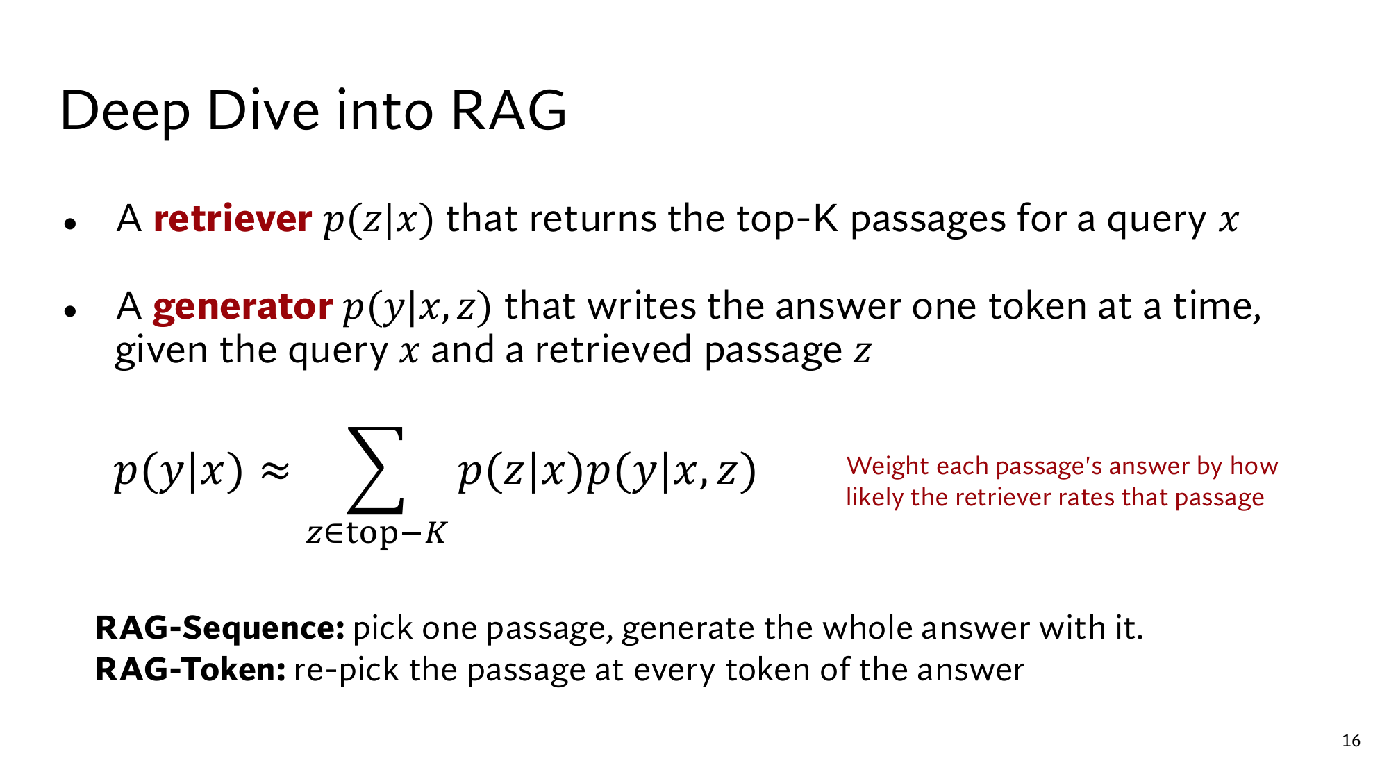
Stanford's slide: Deep Dive into RAG. At the top are the retriever and the generator, in the middle the formula from step 2, and at the bottom the two lines on RAG-Sequence and RAG-Token. You can now read every line of it.
Think first
In the example above, set both passages' weights to 0.5. What probability do RAG-Sequence and RAG-Token give now?
Show the answer
RAG-Sequence: 0.5 × 0.18 + 0.5 × 0.45 = 0.315. RAG-Token: (0.5 × 0.9 + 0.5 × 0.5) × (0.5 × 0.2 + 0.5 × 0.9) = 0.70 × 0.55 = 0.385. RAG-Token is ahead again, because the two tokens still come from different passages.
4Training the retriever and the generator with one loss
RAG's training makes −ln of the right answer's probability small, and this single loss changes both the retriever and the generator. Training all the parts together with one loss is called end-to-end training. The data holds only question-answer pairs, yet this loss is how the retriever learns which passage deserves more weight.
The is the one from lesson 4: −ln of the right answer's probability p. In step 2, Thursday 9am got 0.70, so the loss is −ln 0.70 = 0.357. Over all training examples j, these losses add up:
∑j − log p(yj | xj)
The slide calls this the . It is “marginal” because p(y|x) itself comes from marginalization over passages, and the slide's log is this ln.
Which passage's score lowers the loss when it rises
In the table below, each row raises one score by 0.5 and leaves the other two alone. The weights here have 3 decimals, so the first row's loss is 0.355, not 0.357. my arithmetic
Score raised by 0.5
Weights: queue log, office hours, forum
p(“Thu 9am” | x)
Loss
None
0.602, 0.299, 0.099
0.701
0.355
Queue log, 1.8 to 2.3
0.714, 0.215, 0.072
0.757
0.279
Office hours page, 1.1 to 1.6
0.504, 0.413, 0.083
0.668
0.403
Forum post, 0.0 to 0.5
0.565, 0.281, 0.154
0.664
0.409
When the queue log's score rose, the total probability went from 0.701 to 0.757, and the loss fell. When either of the other two rose, the total fell and the loss rose, even though the office hours page gives 0.5.
The reason lies in the weighted average. p(y|x) is a weighted average of the generator's numbers 0.9, 0.5 and 0.1, meaning each number times its weight, all added up. A weighted average always lies between the smallest and the largest number, and it moves toward whichever number gains weight.
Set the queue log aside for a moment. The office hours page and the forum post have weights in the ratio 3 : 1, that is 0.75 and 0.25 between them. Their average is 0.75 × 0.5 + 0.25 × 0.1 = 0.4. So the total is 0.6 × 0.9 + 0.4 × 0.4 = 0.54 + 0.16 = 0.70. Raising the queue log's score does not change that 3 : 1, because in softmax the other two exps stay the same. So if the queue log's weight is w, the total is w × 0.9 + (1 − w) × 0.4:
Queue log's weight w
Total probability
0.5
0.65
0.6, now
0.70
0.7
0.75
0.8
0.80
1.0
0.90
For the office hours page the same arithmetic runs the other way, because its 0.5 is below 0.79, the average of the other two passages.
The rule: if the generator gives the right answer a higher probability with a passage than the current total, training raises that passage's score. If it gives a lower one, training lowers the score. Here the total is 0.70, so the queue log's score (0.9) goes up, and the scores of the office hours page (0.5) and the forum post (0.1) go down. this rule is not on the slides, it follows from the maths
Now run the same rule on the broken retriever. There the total is 0.27, so both the queue log (0.9) and the office hours page (0.5) go up, and the forum post (0.1) goes down. The queue log was never named in the data, yet training moves the retriever toward it. The last column of the widget in step 2 shows exactly this rule.
Which parts are trained
Training nudges every parameter a little in the direction that lowers the loss, and the gives that direction. Working backwards from the loss to get every parameter's gradient is called backpropagation, or backprop for short. In RAG the gradient reaches the generator's parameters θ and, inside the retriever, the query encoder.
The passage encoder and the index stay fixed. Changing the passage encoder would mean rebuilding the vectors of 21 million passages and then the index. from the paper So training improves things only from the question's side. It changes the query encoder so that q(x) gets larger dot products with the useful passages. If a passage's vector was built badly, training cannot fix it.
The dashed arrow at the top of the slide in step 1 says exactly this: End-to-End Backprop through q and pθ. The arrow reaches q and pθ, not the d(z) in the document index.
Think first
Press “All three equal” in the widget, so each passage has weight 1/3. What is the total probability of Thursday 9am? Which passage's score will training raise, which will it lower, and what happens to the office hours page?
Show the answer
The total is (0.9 + 0.5 + 0.1) ÷ 3 = 0.50. The queue log (0.9) is above it, so its score goes up. The forum post (0.1) is below, so its score goes down. The office hours page gives exactly 0.5, equal to the total, so its score stays where it is.
5Results on NQ: RAG, T5-11B and DPR
The paper measures RAG on question-answering datasets. Natural Questions (NQ) holds real questions people typed into Google search, with answers in Wikipedia. from the paper An answer counts as right only if it matches the correct answer exactly, and this measure is called Exact Match. The score is the percentage of such questions.
The table has two kinds of models. A closed-book model has no documents and answers from its parameters alone. An open-book model first searches documents, then answers.
Model
Kind
NQ
T5-11B
Closed book, 11 billion parameters
34.5
REALM
Open book, picks the answer out of a passage
40.4
DPR
Open book, picks the answer out of a passage
41.5
RAG-Token
Open book, writes the answer itself
44.1
RAG-Sequence
Open book, writes the answer itself
44.5
T5-11B is at 34.5 and RAG-Sequence at 44.5, which is 10 points ahead. Out of 1,000 questions, that is 345 against 445 answers exactly right. So RAG, with documents, gets 100 more questions in 1,000 exactly right than T5-11B with its parameters alone.
The DPR row means the full QA system built on top of the DPR retriever, which picks the answer out of a passage. RAG takes the same kind of retriever, writes the answer itself, and goes from 41.5 to 44.5. RAG-Token is only 0.4 behind RAG-Sequence.
RAG taught its retriever from question-answer pairs, but to do so it also changed the generator's parameters. Today you often get an LLM through a company's API, such as GPT or Gemini, and you cannot change its parameters. Lesson 6 starts from exactly this situation.
From here: the Stanford level
The 5 steps above are the same as in the easy version. The 5 steps below take you to the level of the Stanford slides: first the full maths behind the rule from step 4, then how the same loss reaches the generator and the query encoder. After that come RAG-Sequence and RAG-Token in depth, then the paper's real scale, and finally you read the slides yourself. Every piece of maths is explained where it first appears.
6The maths of the training rule: the loss's rate on a score
The loss's rate on a score tells you how much the loss changes when that score rises a little. Training moves every score against its rate. The rule in step 4 gave only the direction. The rate also tells you how hard each score gets pushed.
A rate: change the input a little, then divide
Finding a rate is simple. Change the input a tiny amount, see how much the output changed, and divide that change by the change in the input. This step uses the exact weights 0.602, 0.299 and 0.099, so the total probability is 0.701 and the loss is 0.355. Now raise one score at a time by 0.01: my arithmetic
Score raised by 0.01
Change in loss
Change ÷ 0.01
Queue log
−0.00171
−0.171
Office hours page
+0.00086
+0.086
Forum post
+0.00086
+0.086
Take an even smaller change than 0.01, and these rates settle at −0.171, +0.086 and +0.085. The number a rate settles at is written ∂𝓛/∂s. The ∂ means that only this one score changed and everything else stayed the same, and such a rate is called a . The minus sign means the loss falls when the queue log's score rises.
The posterior: each passage's share after seeing the answer
These rates come straight out of the table in step 2. Its product column held each passage's share of the total: 0.54, 0.15 and 0.01, out of 0.70. Divide each share by the total: 0.54 ÷ 0.70 = 0.771, 0.15 ÷ 0.70 = 0.214 and 0.01 ÷ 0.70 = 0.014. With the exact weights the same numbers come out as 0.773, 0.213 and 0.014.
These weights after seeing the answer are called the posterior, written p(z|x, y). The retriever's own weights pη(z|x) come before seeing the answer, and they are called the prior. The prior looks only at the question, while the posterior also looks at how easily the right answer comes out with each passage.
p(z|x, y) = pη(z|x) · pθ(y|x, z)p(y|x)
For the queue log the top is 0.602 × 0.9 = 0.542 and the bottom is 0.701, so the posterior is 0.773. p(z|x, y) and pθ(y|x, z) are different things, just as p(full | Tuesday) and p(Tuesday | full) were different in lesson 4.
Now look at the rates: −0.171 = 0.602 − 0.773, +0.086 = 0.299 − 0.213, and +0.085 = 0.099 − 0.014. The loss's rate on each score is exactly prior − posterior.
∂𝓛 / ∂sz = pη(z|x) − p(z|x, y)
The rule from step 4 is hidden in this. Posterior ÷ prior = pθ(y|x, z) ÷ p(y|x). So the posterior is larger than the prior exactly when the generator's number with that passage is larger than the total. For the queue log, 0.9 ÷ 0.701 = 1.284, and indeed 0.773 ÷ 0.602 = 1.284.
Where this rate comes from, in five steps
Write the generator's numbers as az: 0.9, 0.5 and 0.1. Lesson 4's rule for ln and three rules about rates are enough to reach the formula, and every step comes with a check in numbers:
Split the loss into two parts. A softmax weight is es ÷ Z, where Z = e1.8 + e1.1 + e0 = 10.054. So p(y|x) = u ÷ Z, where u = 6.050 × 0.9 + 3.004 × 0.5 + 1 × 0.1 = 7.047. Apply the rule ln(a ÷ b) = ln a − ln b from lesson 4, and 𝓛 = −ln u + ln Z. Check: −1.953 + 2.308 = 0.355.
The rate of es is es itself. Check: (e1.81 − e1.80) ÷ 0.01 = 6.08, about e1.8 = 6.05.
The rate of ln u is 1 ÷ u. Check: (ln 7.057 − ln 7.047) ÷ 0.01 = 0.1418, and 1 ÷ 7.047 = 0.1419.
Linked rates multiply. This is the for rates. When the queue log's score changes, only the term e1.8 × 0.9 inside u changes, at the rate 5.445. When u changes, ln u changes by 1 ÷ 7.047 times as much. So the rate of ln u is 5.445 ÷ 7.047 = 0.773, the queue log's posterior. In the same way the rate of ln Z is 6.05 ÷ 10.054 = 0.602, its prior.
Add the two parts. In 𝓛 = −ln u + ln Z, the queue log's rate is −0.773 + 0.602 = −0.171. The same arithmetic gives prior − posterior for every passage.
One training step on the scores
Training moves each score against its rate. Take a step size of 1, so subtract each score's rate from it: 1.8 + 0.171 = 1.971, 1.1 − 0.086 = 1.014, and 0.0 − 0.085 = −0.085. The new weights are 0.661, 0.254 and 0.085, the total rises from 0.701 to 0.731, and the loss falls from 0.355 to 0.314. my arithmetic
So training pulls the retriever's weights toward the posterior: the queue log's weight went from 0.602 to 0.661, toward its posterior of 0.773. Real training takes this step on parameters, not on scores, which comes in step 7.
In the broken retriever (scores 0, 0.7 and 1.9), the priors are 0.103, 0.208 and 0.689, and the products 0.093, 0.104 and 0.069, which add up to 0.266. The posteriors come out as 0.349, 0.391 and 0.260, so the rates are −0.246, −0.183 and +0.430. The queue log and the office hours page both go up, and the forum post gets the biggest push down.
Think first
With “All three equal”, each prior is 1/3. Work out the posteriors and the rates. What is the office hours page's rate, and why?
Show the answer
The products are 0.300, 0.167 and 0.033, adding up to 0.50. The posteriors are 0.600, 0.333 and 0.067. The rates are 0.333 − 0.600 = −0.267, 0.333 − 0.333 = 0, and 0.333 − 0.067 = +0.267. The office hours page's rate is 0, because its 0.5 equals the total 0.50, and then the posterior stays equal to the prior.
7One loss, two models: rates for the generator and the query encoder
The same loss gives rates to the generator and to the query encoder, and the posterior shows up in both. In step 6 everything happened on the scores. Now see how these rates reach the parameters of both models, and why they do not reach the passage encoder.
The rate for the generator: a push as large as the posterior
The generator's number az is the product of its tokens' probabilities, and by the rule from lesson 4, ln az is the sum of their lns. So a rate on ln az passes straight to every token, and that is the rate to look at. Raise each ln az by 0.01, which means multiplying az by e0.01 = 1.01005: my arithmetic
Which generator number
Rate, from a 0.01 change
Posterior
0.9, with the queue log
−0.774
0.773
0.5, with the office hours page
−0.214
0.213
0.1, with the forum post
−0.014
0.014
The loss's rate on each of the generator's ln az is exactly −posterior. The reason is the same as in step 6. When ln az changes, the term esz az inside u changes at that same rate, and the rate of ln u is 1 ÷ u. Their product esz az ÷ u is the posterior, and the loss holds −ln u, hence the minus sign. Z does not contain az, so that part does not change.
This means the generator learns most to write the right answer with the passage whose posterior is largest. Writing Thursday 9am with the queue log gets a push of 0.773, and with the forum post only 0.014. So the generator does not learn to write Thursday 9am after reading the forum post, which does not contain that fact at all. my reading of the arithmetic, not on the slides
The rate on the query vector, and one step on it
In the retriever the score is d(z)⊤q(x), and training controls only q(x). Now treat q(x) as a real vector with 2 numbers, and give each passage a vector of 2 numbers too. The office hours page keeps its vector from lesson 3. my vectors
Text, and its vector
Dot product with q(x)
Question, q(x)[1.0, 2.0]
–
Queue log, d(z)[1.0, 0.4]
1.0 × 1.0 + 2.0 × 0.4 = 1.8
Office hours page[0.9, 0.1]
1.0 × 0.9 + 2.0 × 0.1 = 1.1
Forum post[0.4, −0.2]
1.0 × 0.4 + 2.0 × (−0.2) = 0.0
If the first number of q(x), q1, rises by 0.01, every score rises by that passage's first number × 0.01. The reason is that in the dot product q1 multiplies only the first numbers. So a score's rate with respect to q1 is the first number of that passage's vector. With the chain rule, the loss's rate with respect to q1 works out like this:
Queue log: score rate −0.171, times its first number 1.0, gives −0.171.
Office hours page: 0.086 × 0.9 = 0.077.
Forum post: 0.085 × 0.4 = 0.034.
Sum: −0.171 + 0.077 + 0.034 = −0.060.
For the second number the same arithmetic gives −0.068 + 0.009 − 0.017 = −0.077. So the loss's rate on q(x) is [−0.060, −0.077], and the formula writes the same arithmetic like this:
∂𝓛 / ∂q(x) = ∑z ( pη(z|x) − p(z|x, y) ) d(z)
Now move q(x) against this rate with a step size of 1: [1.0 + 0.060, 2.0 + 0.077] = [1.060, 2.077]. The new scores are 1.890, 1.161 and 0.009, the weights 0.612, 0.295 and 0.093, the total 0.707, and the loss falls from 0.355 to 0.346.
The office hours page's score also rose, from 1.1 to 1.161, even though its rate said it should fall. All the scores come from the same q(x), so training cannot move them independently. The loss still fell, because the queue log's score rose the most: by 0.090, against 0.061 for the office hours page.
Why the passage vectors stay fixed
The loss also has a rate on d(z). On the queue log's vector it is (prior − posterior) × q(x) = −0.171 × [1.0, 2.0] = [−0.171, −0.342]. In lesson 12, DPR's own training changes the passage encoder with exactly this kind of rate, because no index exists at that point.
RAG does not take this step. If the passage encoder BERTd changed, the vectors of 21 million passages and the index would have to be rebuilt every so often, as REALM does during its pretraining. According to the paper, results were strong without this, so the passage encoder and the index stay fixed. from the paper
From the toy to the real models
In the toy, q(x) itself changed. In reality q(x) = BERTq(x), and carries the same chain rule through every layer of BERTq. The generator's rate reaches every parameter of BART. According to the paper, each BERT encoder has 110 million parameters and BART 406 million, 626 million in total. from the paper The passage encoder's 110 million stay fixed, so training changes about 516 million parameters. my arithmetic
The paper's experiments: freezing the retriever, and swapping in BM25
The paper also measured how much the retriever's learning helps. For this it trained modified models. Such an experiment is called an ablation: remove or freeze one part of the model, and see how far the result drops. In the frozen model the query encoder does not change either. In the BM25 model, lesson 11's BM25 takes DPR's place, and its scores go into the softmax. from the paper
Retriever
RAG-Token
RAG-Sequence
BM25
29.7
31.8
DPR, frozen
37.8
41.2
DPR, learning
43.5
44.0
Exact Match on NQ, on the dev set. That is why these differ a little from the test numbers 44.1 and 44.5 in step 5.
Freezing the query encoder drops RAG-Sequence from 44.0 to 41.2, a loss of 2.8 points. For RAG-Token the drop is 5.7 points.
With BM25, NQ drops by 12 to 14 points: from 44.0 to 31.8, and from 43.5 to 29.7.
On FEVER, where a claim has to be judged true or false from Wikipedia, BM25 did best. The paper's guess is that those claims are full of names, and matching words is what BM25 does.
There is also a risk. In the paper's early experiments, on some tasks such as story writing, the retriever started bringing the same passages for every question. The generator then learned to ignore the passages, and RAG behaved like BART on its own. This is called retrieval collapse. The paper's guess is that with long answers the rates reaching the retriever become weak. from the paper
8RAG-Sequence and RAG-Token in depth: posterior, decoding and K
The difference between the two shows up in the posterior: RAG-Token can keep a different posterior at each token, while RAG-Sequence keeps one for the whole answer. The paper writes the two formulas like this, and in our Thursday-Zoom example N = 2, y1 = Thursday and y2 = Zoom: from the paper
y1:i−1 means tokens 1 through i − 1, the y<i of step 3. For Zoom it is just Thursday. top-k(p(·|x)) is the k passages the retriever brought, here the queue log and the office hours page.
A posterior at every token
In RAG-Token each token has its own weighted sum, so each token also has its own posterior. At Thursday, the queue log's is 0.54 ÷ 0.74 = 0.730 and the office hours page's is 0.20 ÷ 0.74 = 0.270. At Zoom they are 0.12 ÷ 0.48 = 0.25 and 0.36 ÷ 0.48 = 0.75. At the first token the queue log leads, and at the second the office hours page does. RAG-Sequence has a single posterior for the whole answer: 0.108 ÷ 0.288 = 0.375 and 0.180 ÷ 0.288 = 0.625.
The paper's Figure 2 shows the same thing on a real example. In Jeopardy the input was Hemingway, and RAG-Token wrote: "The Sun Also Rises" is a novel by this author of "A Farewell to Arms". While writing Sun, the posterior was high for the passage that mentions The Sun Also Rises, and at A Farewell to Arms it was high for the other passage. After the first token of each title the posterior flattens, because BART completes the rest of the title from its own parameters. from the paper
If the answer is a single token, the two formulas become the same, because the ∏ has just one term left. FEVER's labels, such as supports, are single tokens like this, so there RAG-Sequence and RAG-Token are equal. from the paper
Writing the answer: Thorough and Fast decoding
In training the right answer is known in advance, so computing its probability is enough. At test time the model has to write the answer itself, and this is called decoding. RAG-Token takes the summed probability at each token, such as 0.74 at Thursday, and writes token by token like an ordinary generator. For QA the paper picks the token with the highest probability at each step, the of lesson 1. from the paper
RAG-Sequence's probability does not split into tokens, because its sum comes after the whole answer. So the paper gets its answer in three steps: from the paper
With each passage, the generator writes one answer on its own. These answers are the candidates, and K passages give at most K candidates.
For each candidate, the generator runs again with the passages that did not produce it. This gives the candidate's probability with every passage.
Each candidate gets its weighted sum, and the candidate with the largest sum becomes the answer.
This method is called Thorough decoding. Skip step 2, treating a candidate's probability as 0 with every passage that did not produce it, and you get Fast decoding. On NQ, RAG-Sequence takes 50 passages and runs Thorough decoding, because the answers are short. That means up to 50 candidates, each checked with 50 passages, so up to about 50 × 50 = 2,500 generator runs. For tasks with long answers the paper used Fast decoding, because Thorough did not improve the results. the count of 2,500 is mine
How many passages: the effect of K
In training K was 5 or 10, with no significant difference between the two. At test time the paper picks K itself: for NQ, RAG-Token takes 15 passages and RAG-Sequence 50. The paper's Figure 3 shows that with more passages, RAG-Sequence's NQ score rises and then stays about level. RAG-Token's score peaks at around 10 passages and then falls slightly. from the paper
The second graph in that figure shows answer recall, the percentage of questions with an answer passage inside the top K. At every K the line for RAG's learned retriever sits above fixed DPR, and the BM25 line is far below both. So after end-to-end training the retriever brings the right passages higher, which is the result of step 6.
9The paper's real scale and the full results
Our example had 3 passages and vectors of 2 numbers, so the arithmetic could be done by hand. The paper uses the same mechanism, only with bigger numbers: from the paper
Item
Our example
In the RAG paper
Passages
3
About 21 million pieces of the December 2018 Wikipedia, 100 words each
Vector length
2
768, the BERT-base vectorthis number comes from lesson 12
Index
–
An index in , about 100 GB of CPU memory36 GB when compressed
K
3
5 or 10 in training, 15 (RAG-Token) and 50 (RAG-Sequence) on the NQ test
Models
–
Two BERT-base models with 110 million parameters each, and BART-large with 406 million
Training
By hand
8 GPUs with 32 GB of memory each
NQ questions
1
79,169 for training, 3,611 for testing
On the 3,611 test questions, RAG-Sequence's 44.5 means about 1,607 answers exactly right. Exact Match is strict: it treats Thursday 9 am and Thursday 9am as different. So 44.5 does not mean the other 55.5% of answers were really wrong.
The full results table
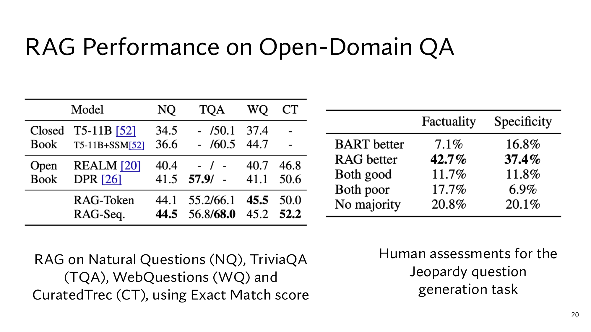
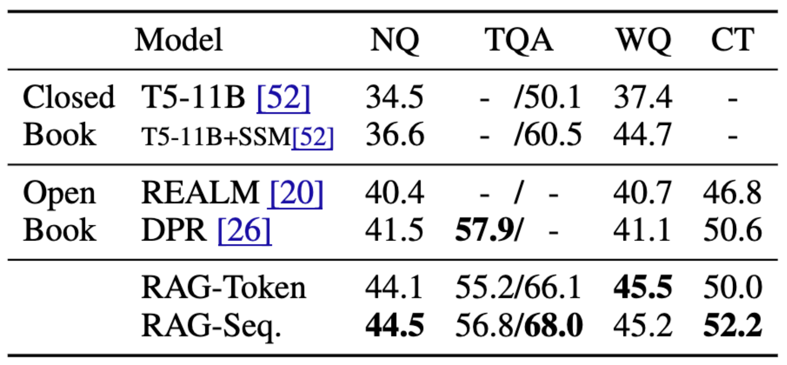
Step 5 showed only the NQ column. The slide's table has four datasets, split here into two tables so that they fit on a phone:
Model
NQ
TQAstandard / Wiki test
T5-11B
34.5
– / 50.1
T5-11B + SSM
36.6
– / 60.5
REALM
40.4
– / –
DPR
41.5
57.9 / –
RAG-Token
44.1
55.2 / 66.1
RAG-Sequence
44.5
56.8 / 68.0
Model
WQ
CT
T5-11B
37.4
–
T5-11B + SSM
44.7
–
REALM
40.7
46.8
DPR
41.1
50.6
RAG-Token
45.5
50.0
RAG-Sequence
45.2
52.2
Exact Match (%) on the test sets. TQA = TriviaQA, WQ = WebQuestions, CT = CuratedTrec.
The largest number in each column is bold on the slide. RAG-Sequence leads on NQ and CT (44.5 and 52.2), RAG-Token on WQ (45.5), and DPR on TQA's standard test set (57.9).
TQA's two numbers belong to two test sets. On the left is the usual open-domain test set, and on the right the Wikipedia one that T5 was measured on. According to the paper the Wiki questions are easier, so RAG-Sequence scores 68.0 there and 56.8 on the usual one.
WQ and CT are small datasets, with only 635 training questions in CT, so the paper started their RAG models from the NQ RAG model. CT's answers are written as regular expressions, so the paper first turned them into plain answers. from the paper
The DPR row is the full DPR QA system. In it, after the retriever, a BERT puts the passages in a new order. Then a reader picks the answer out of a passage. RAG has neither such a reranker nor such a reader, yet on NQ it goes from 41.5 to 44.5. from the paper
According to the paper, one advantage of writing the answer is that passages with clues, but without the answer word for word, still help. On the NQ questions where no retrieved passage held the right answer, RAG still wrote 11.8% of the answers correctly. A model that picks the answer out of a passage would score 0% there. from the paper
REALM and T5-11B + SSM went through a special pretraining called , and RAG did not. But RAG's retriever starts from DPR, which was trained earlier on question-passage pairs from NQ and TriviaQA. So RAG's own training needs no passage labels, but its starting retriever was built from labels.from the paper
The paper gives one more comparison. Among the T5 sizes, the closest to RAG is T5-large with 770 million parameters, and it scores 28.9 on NQ. That is 15.6 points behind RAG-Sequence's 44.5. from the paper
The Jeopardy test
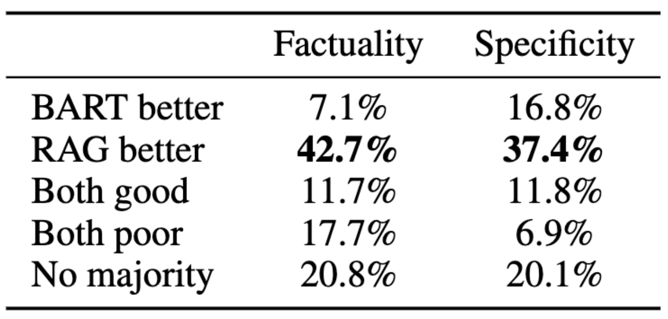
In Jeopardy the answer comes first, and you write a question for it. The paper showed people 452 pairs of questions, one written by BART on its own and one by RAG-Token. In each pair, people chose which question was better: from the paper
People's verdict
Factuality
Specificity
BART better
7.1%
16.8%
RAG better
42.7%
37.4%
Both good
11.7%
11.8%
Both poor
17.7%
6.9%
No majority
20.8%
20.1%
Factuality means a trusted source can back up the statement. Specificity means how tightly the question is tied to its input.
In factuality RAG came out better 42.7 ÷ 7.1 = 6.0 times as often as BART, and in specificity 37.4 ÷ 16.8 = 2.2 times as often. my arithmetic
The factuality column adds up to 100.0, but the specificity column only to 93.0. The paper does not explain the gap. my arithmetic
Jeopardy questions often contain two separate facts, like the two books in the Hemingway question. That is why RAG-Token came out on top here on the paper's automatic measure. from the paper
10Now read Stanford's slides yourself
Below are Stanford's six RAG slides, unchanged. Under each slide are a few questions. Think of the answer first, then open it. If a symbol stops you, go back to the step named in the answer. If a slide looks small on a phone, click the image to open it at full size.
Stanford's RAG slide, and below it the retriever, the generator and the training arrow, enlarged. On the left are three tasks: question answering, fact verification and Jeopardy questions. The REALM and DPR named at the bottom are the open-book rows of the table in step 9.
Read the RAG design slide
The retriever is labelled (Non-Parametric) and the generator (Parametric). The query encoder has parameters too, so why is the retriever called non-parametric?
Show the answer
The retriever's knowledge sits in the passage index, the . The generator's knowledge sits in its parameters θ, its . The query encoder's parameters only decide what comes out of the index. The paper also calls the index the non-parametric memory. (Step 1) from the paper
The dashed arrow at the top stops at q and pθ. Why does it not reach the d(z) in the Document Index?
Show the answer
Training's rates reach the query encoder and the generator. d(z) has a rate too, such as [−0.171, −0.342] on the queue log's vector in the toy, but RAG does not take that step. Changing d(z) would mean rebuilding 21 million vectors and the index. (Steps 4 and 7)
The documents z1 and z2 have a purple part at the bottom, and a line runs to them from the Jeopardy input. What does this show?
Show the answer
The purple part is the input x, in the same colour as the Jeopardy x. The line carries x to every passage, so x and z are concatenated and go into the generator, separately for each passage. (Step 1)
Stanford's two Deep Dive slides. The first has the formula and the two lines at the bottom, the second has the training line. Their key parts are enlarged below each. Every symbol of the formula is covered in lesson 4's dense version.
Read the Deep Dive slides
The RAG-Sequence line says pick one passage. Does RAG-Sequence really pick one passage and drop the rest?
Show the answer
No. It writes the whole answer with every passage and takes the weighted sum of all of them: 0.6 × 0.18 + 0.4 × 0.45 = 0.288. Pick one passage means the whole answer rests on a single passage, so the whole answer has one posterior, 0.375 and 0.625. (Steps 3 and 8)
The red note says to weight each passage's answer by how much the retriever trusts that passage. What does that trust look like after seeing the answer, and what does training do with it?
Show the answer
The formula's trust is the prior p(z|x). The trust after seeing the answer is the posterior, 0.773 instead of 0.602 for the queue log. Training pulls the prior toward the posterior, because the loss's rate on a score is prior − posterior. (Step 6)
The second slide says Jointly train the retriever and generator. Which part of the retriever is really trained?
Show the answer
Only the query encoder BERTq. The passage encoder BERTd and the index stay fixed, while the generator BART is trained in full. About 516 million of the 626 million parameters change. (Steps 4 and 7)
In the training line, what does ∑j run over, and how many j are there for NQ? Does any j name a passage?
Show the answer
It runs over every training pair (xj, yj). NQ has 79,169 training questions, and the paper turns every correct answer of a question into a separate pair, so there are even more j. No pair names a passage, which is why p(yj|xj) comes from marginalization over passages. (Steps 2, 4 and 9) from the paper
Stanford's retriever and generator slides, with their parts enlarged.
Read the retriever and generator slides
Where do BERTd and BERTq come from, and which of them changes in RAG's training? How does this differ from DPR in lesson 12?
Show the answer
Both come from DPR, which was trained earlier on question-passage pairs from NQ and TriviaQA. In RAG only BERTq changes. In DPR's own training both change, because no index exists at that point. (Steps 7 and 9) from the paper
What is the k in top-k(p(·|x))? What value does it take in training and on the NQ test?
Show the answer
k is the number of passages brought, the K of the earlier slides. It is 5 or 10 in training, and on the NQ test 15 for RAG-Token and 50 for RAG-Sequence. (Step 8)
The generator slide says x and z are concatenated, and also that any encoder-decoder will do. How do these two points connect to the RAG formula?
Show the answer
The formula needs only pθ(y|x, z) from the generator. BART reads a single text, so x and z are joined into one input, like the queue-log input in step 1. With K passages there are K separate inputs. Any encoder-decoder that gives this probability can take that place. (Steps 1 and 2)
The generator writes one token at a time. With K passages, how does it write the answer in RAG-Token and in RAG-Sequence?
Show the answer
In both, the generator runs separately with each passage, on K inputs. RAG-Token adds the K passages' probabilities at every token and writes a single answer. RAG-Sequence writes a separate answer with each passage, and Thorough decoding then checks every candidate again with the other passages. (Step 8)
Stanford's results slide, and below it both tables, enlarged.
Read the results slide
DPR (41.5) and RAG-Seq. (44.5) use the same kind of retriever. Where does the difference come from?
Show the answer
The DPR system picks the answer out of a passage, and it also has a reranker. RAG writes the answer itself, and its query encoder was trained further on the answer's loss. Even on questions where no passage held the answer, RAG wrote 11.8% correctly. (Steps 5, 7 and 9)
In the WQ column the bold 45.5 belongs to RAG-Token. Does this mean RAG-Token is clearly better for WQ?
Show the answer
The gap is only 45.5 − 45.2 = 0.3. WQ's test set has 2,033 questions, so 0.3% is about 6 questions, and a gap that small is hard to call real. (Step 9) my arithmetic
Add up both columns of the right-hand table. What do you get, and what does the table say about RAG?
Show the answer
Factuality: 7.1 + 42.7 + 11.7 + 17.7 + 20.8 = 100.0. Specificity: 16.8 + 37.4 + 11.8 + 6.9 + 20.1 = 93.0, and the paper does not explain why. In both columns the largest row is RAG better: in factuality RAG came out better 6.0 times as often as BART. (Step 9)
3 points from this lesson
RAG treats the passage as a hidden choice and takes a weighted sum over the top-K passages: p(y|x) ≈ ∑ pη(z|x) · pθ(y|x, z). So RAG's own training needs no labels for the right passage.
The loss's rate on each score is prior − posterior, and on each of the generator's ln az it is −posterior. So training pulls the retriever's weights toward the posterior, and the generator learns most with the passage whose posterior is large.
RAG-Token can keep a different posterior at each token, while RAG-Sequence keeps one for the whole answer. The query encoder and the generator are trained, the passage encoder and the index are not. Even so, the learned retriever beats a frozen one by 2.8 points on the NQ dev set, and BM25 by 12.2.
New terms in this lesson
RAG
Retrieval-Augmented Generation: joining a retriever and a generator into one model and training them together with one loss. For example, bringing the queue log and writing Thursday 9am from it.
Latent variable
A hidden choice that the data does not record. In RAG, the choice of which passage the answer came from. For example, a question-answer pair does not say that the answer came from the queue log.
η and θ
The names of the retriever's (eta) and the generator's (theta) parameters. That is why the retriever is written pη(z|x) and the generator pθ(y|x, z).
BERT
An encoder model Google released in 2018. Both of the RAG retriever's encoders, the query encoder and the passage encoder, are built from it.
MIPS
Maximum inner product search: finding the K passages in the index with the largest dot products. For example, the 5 highest scores among 21 million passages.
Generator
The model that reads the question and one passage and writes the answer, pθ(y|x, z). In RAG it is BART. For example, 0.9 for Thursday 9am with the queue log.
Encoder-decoder
The encoder turns the input into vectors, and the decoder looks at them while it writes one token at a time. BART is such a model.
Concatenate
Join two texts end to end into one text. For example, question: … followed by passage: ….
RAG-Sequence
The whole answer with each passage, then the weighted sum. For example, 0.6 × 0.18 + 0.4 × 0.45 = 0.288.
RAG-Token
A weighted sum at every token, then the product of the tokens. For example, 0.74 × 0.48 = 0.355.
End-to-end training
Training all the parts together with one loss. In RAG the query encoder and the generator both learn from the same −ln p(y|x). For example, −ln 0.70 = 0.357.
Backpropagation
Working backwards from the loss to get every parameter's gradient, backprop for short. In RAG it reaches the generator and the query encoder, but not the passage encoder.
Exact Match
An answer counts as right only if it matches the correct answer exactly. The score is the percentage of such questions. For example, RAG-Sequence's 44.5 on NQ.
Closed book and open book
Answering from parameters alone, or searching documents first and then answering. For example, on NQ the closed-book T5-11B scores 34.5 and the open-book RAG-Sequence 44.5.
Posterior and prior
The prior pη(z|x) is a passage's weight before seeing the answer, and the posterior p(z|x, y) is its weight after, that passage's share of the total probability. For example, the queue log's prior is 0.602 and its posterior 0.773.
Ablation
Removing or freezing one part of a model and measuring again, to see what that part contributes. For example, freezing the query encoder in RAG-Sequence drops NQ (dev) from 44.0 to 41.2.
Thorough and Fast decoding
Two ways for RAG-Sequence to write an answer. Each passage produces one candidate. Thorough checks every candidate with every passage, Fast only with the passage that produced it. For example, with 50 passages on NQ, Thorough needs up to about 2,500 generator runs.
Retrieval collapse
The retriever starts bringing the same passages for every question during training, after which the generator learns to ignore them. For example, on the paper's story-writing task.