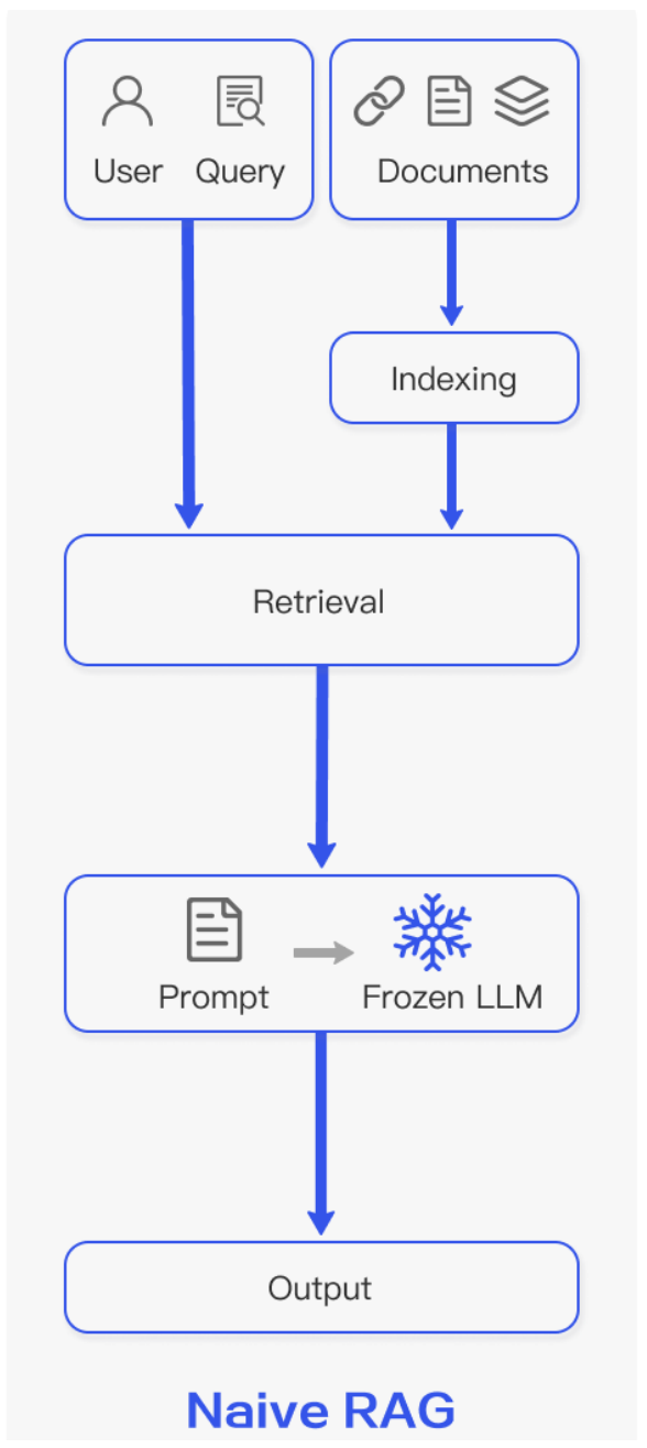
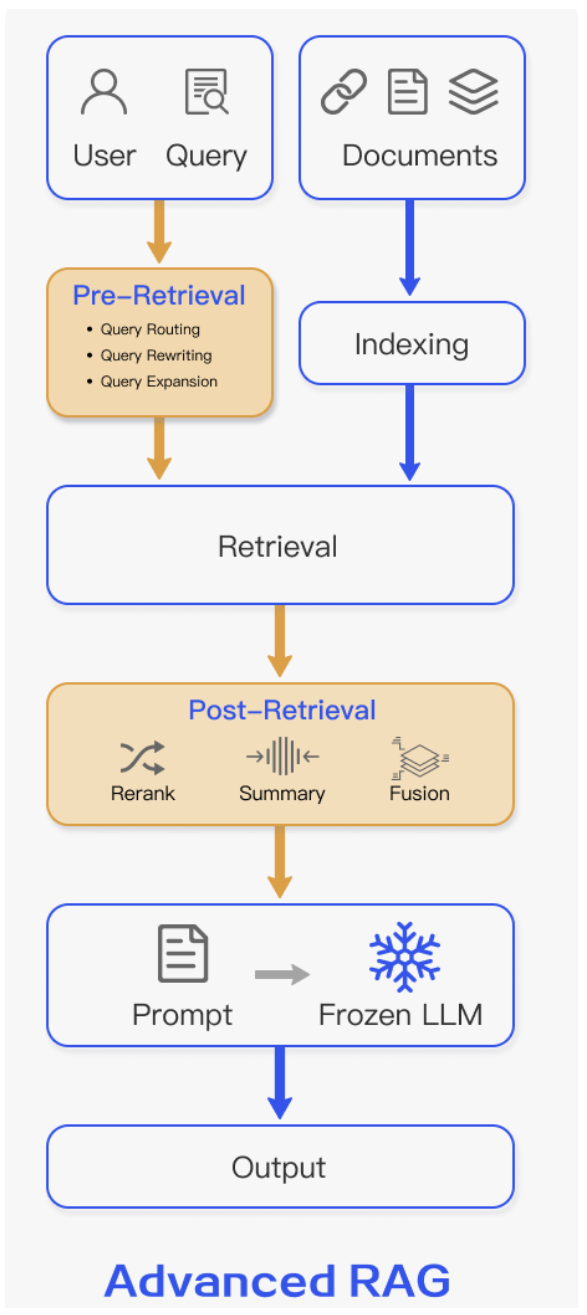
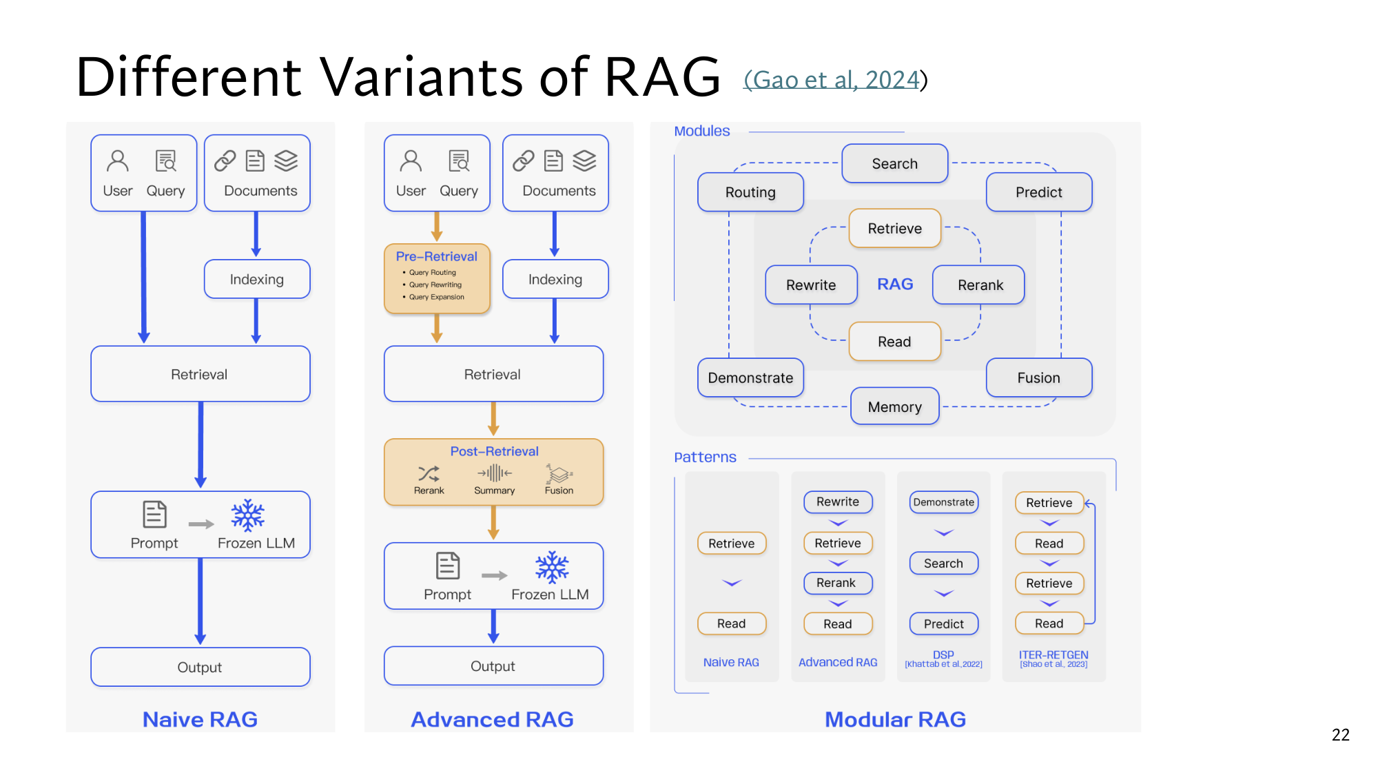
A RAG pipeline is a line of steps: from the query to retrieval, from retrieval to the prompt, and from the prompt to the LLM's answer. You cannot change the LLM, so to improve the answer you change the steps before it. Stanford's slide shows three forms of such a pipeline: Naive, Advanced and Modular RAG.
The need for this showed up at the end of lesson 5. There the retriever and the generator were trained together. But you cannot change the parameters of an LLM you use through an API, such as GPT or Gemini. Then both mistakes from lesson 2 come back. For when can I get help from a TA, the retriever returns no passage at all. For which office hour is least crowded, the old forum post gets the same score as the queue log.
The ladder for this lesson
The ladder has 10 steps. The first 5 are the same as in the easy version, and steps 6 to 10 take you to the level of the Stanford slides. Under each step you can see what you will be able to do after it.
What you need first: Lesson 2 (retriever, word overlap, stopwords, recall ceiling), Lesson 3 (embedding, index) and Lesson 5 (the RAG model, concatenate, Exact Match). Step 9 also uses Lesson 4 (conditional probability, chain rule). If you already know a step, skip to the next one. A word with a dotted underline and ▾ opens its definition when you click it.
1The frozen LLM: you can only change the prompt
A frozen LLM is an LLM whose parameters you cannot change. You can only send it a prompt and get an answer back. The of an LLM behind an API sit on the company's servers, so for you that LLM is frozen.
Lesson 5's RAG cannot be trained in this setting. There, used a single loss to change the parameters of both the retriever and the generator. A frozen LLM's parameters cannot change at all, so that route is closed.
What you can still change is everything before the LLM: the query, the retriever and the prompt. A pipeline is a line of steps in which the output of each step becomes the input of the next. For example, the retriever's output is the top-K passages, and those passages become the input of the prompt.
In a pipeline, the top-K passages all go into one prompt. In lesson 5 the generator ran separately with each passage, and the results were combined as a weighted sum. Here the LLM gets a prompt like this: my example
Answer using only the passages below. Cite passage IDs. [P3] Queue log, last 3 weeks: Tuesday 4pm office hour averaged 14 students waiting; Thursday 9am office hour averaged 3. [P2] Office hours: Tuesday 4pm in Room 104 and Thursday 9am on Zoom, run by the TAs. Question: Which office hour is least crowded, and where is it?
The LLM itself picks which fact to take from which passage: Thursday 9am from the queue log, and Zoom from the office hours page. [P3] and [P2] are passage IDs from lesson 2's corpus, so the answer can cite them.
The price of this freedom is that the LLM learns nothing from its mistakes, and the retriever never even finds out about them. We are back to lesson 2, where the retriever and the reader were built separately. So every step has to be made good on its own, and the rest of this lesson shows those steps.
2Naive RAG: indexing time and query time
Naive RAG is the simplest pipeline: an index built in advance, and then retrieval, a prompt and the frozen LLM for every query. There is no extra step in between, which is why it is called naive, meaning plain. Its steps split into the same two parts that were in lesson 3.
In pipeline terms these two parts are called indexing time and query time. The indexing-time steps run once: split the documents into passages, make an of each passage, and store them all in an . An embedding is the vector an encoder makes from a piece of text.
Documents2,000 documents
Split into passages60,000 passages
Index60,000 embeddings, once
Indexing time: this line runs once. The numbers come from lesson 2's company: 2,000 documents × 30 paragraphs = 60,000 passages. my example
The query-time steps run for every query:
Query1 embedding
Retrieve60,000 dot products, top-5
Prompt5 × 500 tokens + the question
Frozen LLMRead, 1 call
Query time: this line runs for every query. my example
So every query costs 1 embedding, 60,000 and 1 LLM call. The prompt carries 5 × 500 = 2,500 tokens of passages. The two main query-time steps are called Retrieve and Read. In Read, the LLM reads the passages and writes the answer, like the in lesson 2.
The left part of Stanford's slide: Naive RAG. From Documents to Indexing is indexing time, and from Query to Output is query time. The snowflake next to Frozen LLM marks it as frozen. Click the image to open it at full size.
Now run the two opening questions through this pipeline. For the retriever we use from lesson 2, because you can count every score by hand. Word overlap counts how many of the query's words also appear in a passage, and it first removes such as which and is.
Query
What the retriever returned
What the LLM got at K = 2
when can I get help from a TA
Nothing. Every passage scores 0.
Nothing. The office hours page, which has the answer, never reached the LLM.
which office hour is least crowded
Queue log (2), old forum post (2), office hours page (1)
The queue log and the forum post: the real data plus an old opinion from 2024
The two mistakes are of different kinds. For the TA question the right passage never came back, and that is lesson 2's . For the least-crowded question the right passage came back, but a wrong passage came along with the same score, so this is a mistake in the order. Both mistakes happen before anything reaches the LLM, so no LLM, however good, can fix them.
Think first
500 new passages are added to the corpus, and one old document changes. Which Naive RAG steps have to run again, and which do not?
Show the answer
Only the indexing-time steps, and only for the text that changed. Make embeddings for the 500 new passages and add them to the index, and remake the embeddings of the changed document's passages. If you skip this, the index keeps returning the old text. The query-time steps run as before, and nothing changes in the LLM.
3Pre-retrieval: improving the query before retrieval
Pre-retrieval is the set of steps that improve the query before it goes to the retriever. The slide gives three of them: query routing, query rewriting and query expansion. Start with expansion on the TA question, because that question failed on the words of the query.
Without stopwords, this query keeps help and ta. The office hours page says TAs, not ta, and word overlap only matches exact words. Help appears in no passage. So the answer's passage is in the corpus, and only the query's words fail to match it.
Query expansion adds related words to the query, so that it can match the words in the passages. Add office hours to the TA query, and the retriever has four words: help, ta, office and hours. my example
Passage
Matching words
Before expansion
After expansion
Office hours page
office, hours
0
2
Queue log
office It says hour, not hours.
0
1
The other four passages
none
0
0
Now the office hours page is on top and reaches the LLM. The added words usually come from an LLM given a short prompt: write search words related to this question.
The other two steps also work on the query. Query rewriting writes the whole query again. If a user types the short form OH timings?, an LLM turns it into CS 329Z office hours schedule. Query routing decides which index to search. For example, when is the project milestone due should go to the syllabus index.
Switch the pipeline's steps on and off
The retriever is lesson 2's word overlap. Expansion adds words to the query. Rerank sorts the returned passages again by a second score, and it comes in the next step. my rerank scores
#
Passage
Overlap
Rerank
These steps have a cost. Rewriting and expansion usually need one extra LLM call per query, so the answer is slower and more expensive. They can also change what the query means: if the model reads OH as Ohio, the search goes to the wrong place.
Think first
Pick which office hour is least crowded in the widget. Expansion adds waiting to this query. What are the new scores of the queue log and the old forum post? Then check in the widget.
Show the answer
The query's words are now office, hour, least, crowded and waiting. The queue log has office, hour and waiting, so it scores 3. The forum post has least and crowded, so it scores 2. The queue log is now alone at the top, but at K = 2 the forum post still goes into the prompt.
4Post-retrieval: improving the returned list
Post-retrieval is the set of steps that improve the retriever's list before it goes into the prompt. The slide gives three of them: rerank, summary and fusion. Start with reranking on the least-crowded question, because there the mistake was in the order.
The retriever gave the queue log and the forum post the same score, 2. It cannot see that the queue log is three weeks of data while the forum post is a single opinion from 2024.
The retriever is fast because it looks at every passage only roughly. The returned passages are few, so a slower but more accurate model can look at them. This model reads the query and the passage together, gives the passage a new score, and sorts the list again. This is called reranking, and the model is a reranker. How a reranker is built comes in lesson 14.
The retriever returned three passages, and the reranker puts the forum post at the bottom: my rerank scores
Passage
Retriever score
Reranker score
Reaches the LLM at K = 2?
Queue log
2
0.92
Yes
Office hours page
1
0.41
Yes
Old forum post
2
0.35
No
At K = 2 the queue log and the office hours page now go through, and this pair gives the full answer. The queue log says Thursday 9am is the least crowded, and the office hours page says it is on Zoom. This is the prompt shown in step 1.
Think first
Pick the TA query in the widget. Leave Expansion off and turn Rerank on. Does the office hours page reach the LLM now?
Show the answer
No. The retriever returned no passage at all, so the reranker has nothing to sort. Now turn Expansion on as well: the office hours page enters the list, and reranking puts it on top.
A reranker only changes the order of the passages the retriever returned. So the two kinds of steps fix different mistakes. Pre-retrieval brings a missed passage into the list, and post-retrieval fixes the order of the list.
Two more steps come after retrieval. The first is summary: shortening the passages before they go into the prompt. Lesson 1's context window had room for 7,000 tokens of passages, which is 14 passages of 500 tokens. If each passage shrinks to 100 tokens, the same 14 passages take 14 × 100 = 1,400 tokens. my example The risk is that the summary drops a detail that matters, such as Room 104.
The second is fusion: merging several ranked lists into one. Suppose you searched with the original query and also with the rewritten query office hours schedule. The first list is queue log, forum post, office hours page. The second has only the office hours page (2) and the queue log (1). Those two passages appear in both lists, so they should rise to the top of the merged list. The exact way to merge comes in lesson 14.
The pipeline you get by adding pre-retrieval and post-retrieval steps to Naive RAG is called Advanced RAG.
The middle part of Stanford's slide: Advanced RAG. The orange boxes are the new steps: the three Pre-Retrieval steps above Retrieval, and the three Post-Retrieval steps below it.
5Modular RAG: modules and patterns
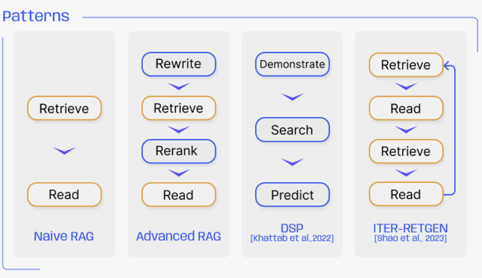
Modular RAG sees the pipeline as modules that you can connect in any order. A module is one part of the pipeline that does one job, such as Retrieve, Rerank or Read. A fixed order of modules is called a pattern. Naive RAG's pattern, for example, is Retrieve, then Read.
This matters for questions whose answer is spread over several passages. Advanced RAG still searches only once per question, so whatever the first search misses never arrives. A question that needs more than one search is called a multi-hop question.
Our corpus has such a question too: the one from the prompt in step 1, Which office hour is least crowded, and where is it? The first part of the answer is in the queue log, and the second part is in the office hours page. The office hours page gives the place next to Thursday 9am, so to find it you first need to know that the answer is Thursday 9am.
Now run the pattern Retrieve, Read, Retrieve, Read, in which the answer from the first Read is added to the query of the second search. K is 2, and the retriever is the same word overlap. my example
First Retrieve: the query keeps office, hour, least, crowded and where, and where appears in no passage. The queue log and the forum post score 2 each, so those two come back.
First Read: suppose the LLM goes with the queue log's data and writes: Thursday 9am. Neither passage says where it is.
Second Retrieve: put the first answer, Thursday 9am, in front of the query. Now thursday and 9am count too.
Second Read: at K = 2 the LLM gets the queue log and the office hours page, which is the prompt from step 1. It writes: Thursday 9am, on Zoom.
Passage
First search
Second search
Queue logoffice, hour, then also thursday, 9am
2
4
Office hours pageoffice, then also thursday, 9am
1
3
Old forum postleast, crowded
2
2
Syllabusthursday, the second time
0
1
This pattern is called ITER-RETGEN. Its paper also builds the next query by joining the previous answer to the question. from the paperReranking only changes the order of the returned list, while ITER-RETGEN searches again with a new query.
It has a limit too. If the first Read gets the answer wrong, the second search heads the wrong way. If the LLM trusts the forum post and writes Wednesday, Thursday 9am never enters the second query.
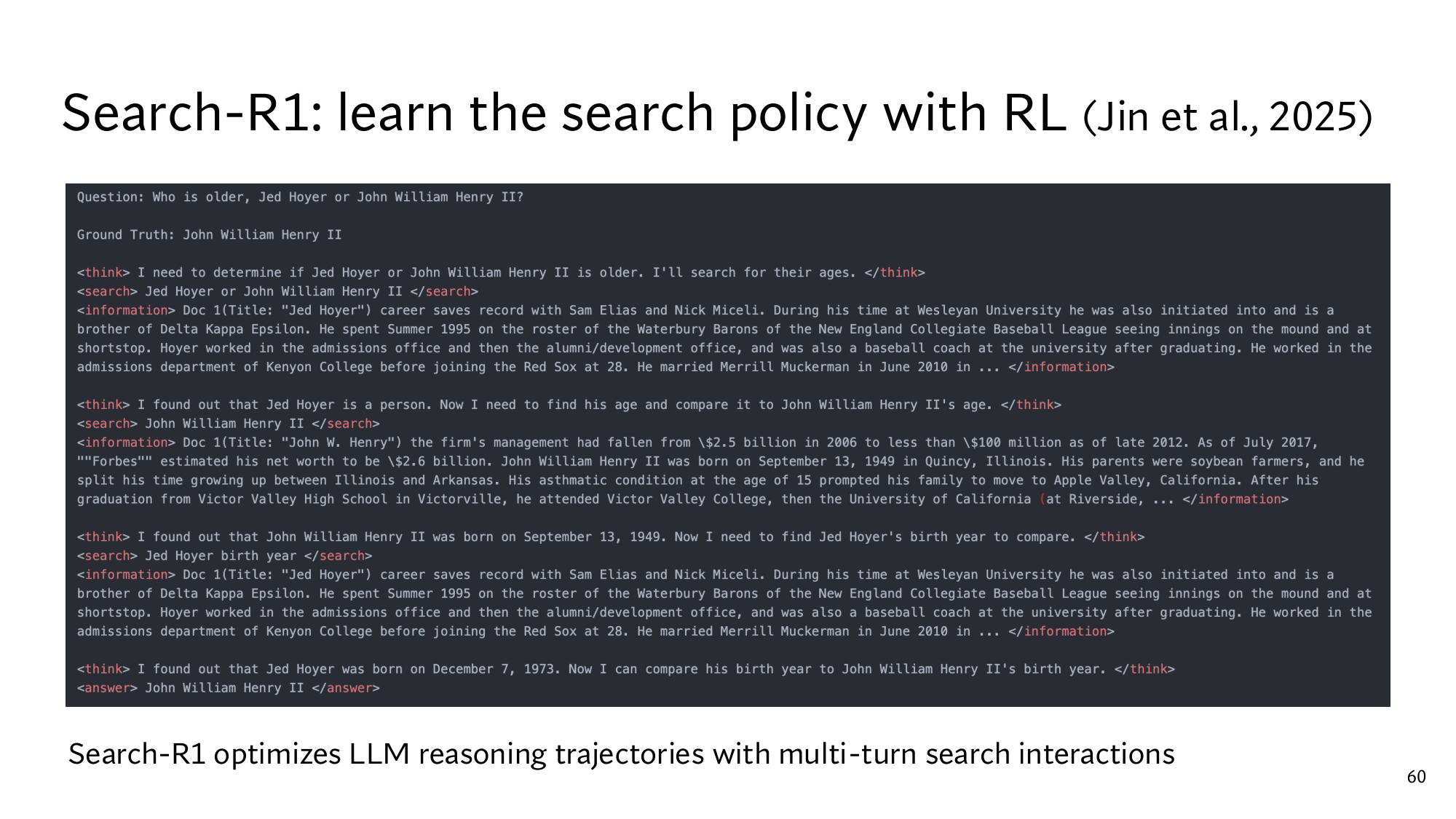
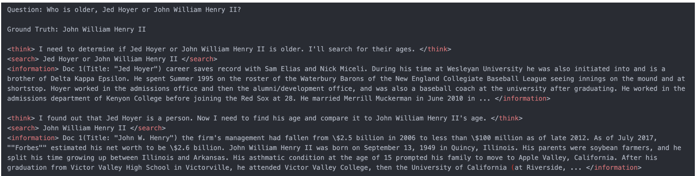
The lecture also has a real multi-hop question: Who is older, Jed Hoyer or John William Henry II? The slide shows a model's trace on this question, which lesson 17 covers in full. The first search returns a passage about Jed Hoyer's career, with no date of birth in it. The next search is for John William Henry II, and its passage says: born September 13, 1949. The third search is for Jed Hoyer birth year, so each search depends on what the previous reading found.
Stanford's slide: the trace of a model called Search-R1. The <search> lines are the model's searches, and the <information> lines are the passages that came back.
Stanford's slide shows four patterns, taken from the survey by Gao and colleagues (2024):
DSP's Demonstrate module puts a few worked examples in the prompt before the question, such as Q: When is the milestone due? A: Week 6, Thursday [P1]. my example Such examples are called demonstrations, and the method is called few-shot prompting. It differs from lesson 2's setup, where the prompt held only an instruction.
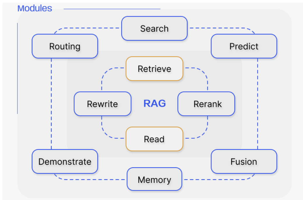
The modules part of the slide has 10 modules, and you have now seen 7 of them. The other three, Search, Predict and Memory, come in the dense version.
The right part of Stanford's slide: Modular RAG. The modules are at the top, and the four patterns below. In ITER-RETGEN, the arrow from the last Read back to the first Retrieve says that the sequence runs again.
A person writes the pattern in advance, so in ITER-RETGEN the number of searches is fixed, whether the question needs 1 search or 3. In lesson 16 and 17, the model itself decides when the loop stops and what the next query is. Every extra loop adds one more LLM call.
From here: the Stanford level
The 5 steps above are the same as in the easy version. The 5 steps below take you to the level of the Stanford slides: first Naive and Advanced RAG as the survey describes them, then all of the slide's modules, then the DSP and ITER-RETGEN papers, and finally reading both slides yourself. Every piece of maths is explained where it first appears.
6Naive and Advanced RAG in the survey: three problems, precision and sets
The diagram on Stanford's slide comes from a survey by Gao and colleagues. A survey is a paper that reads many papers in a field and arranges them into one framework. This one sorted more than 100 RAG papers into three forms: Naive, Advanced and Modular RAG. from the paper
Naive RAG's three stages and three problems
The survey describes Naive RAG in three stages: indexing, retrieval and generation. It also calls this the Retrieve-Read framework. In indexing, documents in formats such as HTML, Word and Markdown are first turned into plain text. The text is then split into chunks, and each chunk's embedding goes into a vector database. from the paper
In retrieval, the query's embedding is made by the same encoder that made the chunks' embeddings. Otherwise the query vector and the chunk vectors would be built in different ways, and their dot product would mean nothing. In generation, the query and the chosen chunks go into one prompt, just as in step 1.
The survey then lists three problems with Naive RAG. Each one comes with an example from our corpus below: my examples
Problem
What the survey says
In our corpus
Retrieval
Low precision and low recall: wrong chunks come back, and needed chunks are missed.
At K = 2 the forum post came back, and for the TA question the office hours page was missed.
Generation
Hallucination: the answer says something the returned text does not support.
The LLM writes that the Thursday 9am office hour is in Room 104, while the passage says Zoom.
Augmentation
Combining passages is hard: when several passages say the same thing, the answer repeats itself.
The queue log and the office hours page both mention Tuesday 4pm and Thursday 9am.
The first row brings a new word, precision. Precision is the share of the returned passages that are right. For the least-crowded question at K = 2, the queue log is right and the forum post is wrong, so precision = 1 ÷ 2 = 0.5. Recall counts from the other side: how many of the needed passages came back. For the TA question one passage was needed and none came back, so recall = 0 ÷ 1 = 0.
The survey adds a fourth point: for a hard question, one search with the original query is often not enough. from the paper The multi-hop question in step 5 is exactly this problem.
In the language of sets: expansion never lowers a score, and reranking never adds a passage
Two claims from steps 3 and 4, the limits of expansion and of reranking, can be proved cleanly with sets. A is a group of things in which each thing appears once. It is written in curly brackets, so the set of words in the TA query is Q = {help, ta}. The number of things in a set is written with bars: |Q| = 2.
The things two sets have in common form their intersection, written ∩. The least-crowded query's set is {office, hour, least, crowded}. Its intersection with the queue log's words is {office, hour}, which holds 2 things. The word overlap score is exactly this count:
score(Q, P) = | Q ∩ P |
Here Q is the set of the query's words, and P is the set of the passage's words. For the queue log |{office, hour}| = 2, and for the forum post |{least, crowded}| = 2.
Putting two sets together into one is called their union, written ∪. That is what expansion does: it joins a set E of related words to the query's set Q. For the TA query, Q ∪ E = {help, ta} ∪ {office, hours} = {help, ta, office, hours}. For the office hours page, Q ∩ P was empty, and (Q ∪ E) ∩ P = {office, hours}.
Now the proof. A word in Q ∩ P is in Q and also in P. Every word of Q is also in Q ∪ E, so that word is in (Q ∪ E) ∩ P as well. So everything in the old intersection is still in the new one, and new things can join:
| (Q ∪ E) ∩ P | ≥ | Q ∩ P |
So expansion can never lower any passage's word overlap score. That is its strength, because a missed passage can rise. It is also its limit, because a wrong passage never drops either. After adding waiting, the forum post stayed at 2.
For reranking, call the set of returned passages R and the set of needed passages G. Reranking only changes the order of the things in R, so R stays the same, and so does |R ∩ G|. For the TA question R = { }, the empty set, and it is still empty after reranking. Reranking does not change recall. It can only change the precision of the top K. In step 4, at K = 2 the forum post was in the top two at first. After reranking, the office hours page took its place, and that page is needed for the where part.
The survey's other pre-retrieval and post-retrieval methods
On the slide, pre-retrieval holds only the three query steps. The survey also counts improving the index as pre-retrieval, and lists several forms of each step: from the paper
Improving the index: choosing the chunk size, sliding windows, and , which is extra information stored with a chunk, such as a date. The survey says that weighting by date keeps the retriever away from outdated information. Our forum post is marked 2024, so such a weight would push it down. Chunks come in lessons 7 and 8.
Forms of expansion: Multi-Query makes several queries from one and runs them together. Sub-Query breaks a hard question into smaller questions. In Chain-of-Verification, the LLM checks the expanded queries.
Forms of transforming the query: you saw Rewrite in step 3. In HyDE, the LLM first writes a made-up answer, and the embedding of that answer is used to find real passages. Step-back also writes a more general form of the question, and searches with both. The survey's example: LLM can mean large language model, or a law degree.
Forms of routing: a metadata router pulls names or keywords out of the query and filters chunks by their metadata. A semantic router chooses the route by the query's meaning.
Rerank: by rules, or with a model. The survey gives one more piece of advice: put the most useful text at the edges of the prompt. The reason is that an LLM pays less attention to the middle of a long text. This is called , and it comes in lesson 18.
Shrinking the context: adding more documents adds more noise. Methods such as LLMLingua use a small model to remove the less useful tokens.
In the summary example, each passage went from 500 to 100 tokens, so it became 500 ÷ 100 = 5 times smaller. Then the same 7,000 tokens of room fit 7,000 ÷ 100 = 70 passages instead of 14. my arithmetic So a summary can either raise K, or make every query cheaper.
7All the modules of Modular RAG, and the survey's new patterns
The modules part of the slide has two rings. The inner ring, around the word RAG, holds Retrieve, Rewrite, Rerank and Read, the modules of the Advanced RAG pattern. The outer ring holds Search, Routing, Predict, Demonstrate, Memory and Fusion. The dashed lines say that modules can connect to each other in any order.
The Retrieve and Read boxes have orange borders, and the rest have blue ones. The patterns part uses the same colours, so orange probably marks Naive RAG's two original modules. my guess The table below shows what each module does on our corpus:
Module
Job
In our corpus
Retrieve
Top-K passages from the index
Word overlap, K = 2
Read
Read the passages and answer
Thursday 9am, on Zoom
Rewrite
Write the query again
OH timings? becomes CS 329Z office hours schedule
Rerank
Sort the returned list again
The forum post at 0.35, at the bottom
Routing
Pick the source or route
The milestone question goes to the syllabus index
Fusion
Merge several lists
The queue log and the office hours page rise from two lists
Demonstrate
Worked examples in the prompt
The milestone Q and A
Search
Search a search engine, database or knowledge graph directly
If office hours lived in a database table, the LLM would write a query for it
Predict
The LLM writes the context itself instead of retrieving it
The LLM writes CS 329Z's office hours from memory
Memory
Text the LLM wrote earlier guides the next retrieval
The first Read's Thursday 9am goes into the next search
The job column follows the survey. The corpus examples are mine.
According to the survey, the Search module also has the LLM write code or a query language, so that it can search sources such as databases. The Predict module aims to cut down repetition and noise in what retrieval returns. But our course's office hours were never in any LLM's training, so here Predict would make up a wrong answer. The survey also lists a Task Adapter module, which is not on the slide. It adapts RAG to a particular task. from the paper
In Modular RAG the order of the modules can change too. The survey lists some new patterns: from the paper
Rewrite-Retrieve-Read: the query is rewritten first. The model that rewrites learns from feedback on the LLM's answers.
Generate-Read: instead of retrieving, the LLM writes the text itself, which is the Predict module.
Recite-Read: the model “recites” knowledge from its own parameters, then reads that to write the answer.
Hybrid retrieval: combining word-based search with vector search. This comes in lesson 14.
DSP and ITER-RETGEN: one module's output improves another module's work. Both are on the slide, and the next two steps cover their papers.
8DSP: passing text between a frozen LM and a retriever
DSP, short for Demonstrate–Search–Predict, is a program that solves hard questions by passing text back and forth between a frozen LM and a frozen retriever. Khattab and colleagues at Stanford built it in 2022. The paper uses GPT-3.5 as the LM, short for language model, and ColBERTv2 as the retriever. Neither is trained. from the paper
The paper's first example is this question: How many storeys are in the castle David Gregory inherited? It needs the castle's name first, and then its number of storeys. Three systems handle it differently: from the paper
The LM alone invents a castle called Castle Gregory and says it has three storeys.
Retrieve-then-read, that is, Naive RAG, searches with the question itself and finds a passage about the St. Gregory Hotel. The answer comes out as nine storeys.
DSP: the LM writes a first query, Which castle did David Gregory inherit?, and the passage says Kinnairdy Castle. The second query asks for that castle's storeys, and the answer comes back: five storeys.
DSP has three stages, and the slide has a module for each: from the paper
Demonstrate: the program has a few question-answer pairs, such as 16, but no labels for the queries in between. It runs Search and Predict on these training questions itself. Whenever its answer matches the correct answer, the whole path, meaning the queries and passages, becomes a demonstration.
Search: the LM writes the query for each hop, and the retriever brings its passages. On the multi-hop dataset HotPotQA the number of hops is fixed at 2.
Predict: the LM reads the demonstrations and the passages and writes the final answer.
Here is the Demonstrate stage on our corpus. The training pair is the question when is the project milestone due, with the answer Week 6, Thursday 11:59pm. my example
Search: the query keeps project, milestone and due. The syllabus scores 3, and the project page scores 2.
Predict: reading the syllabus, the LM writes Week 6, Thursday 11:59pm. This matches the correct answer.
So the whole path, the question, the syllabus and the answer, becomes a demonstration. Had the answer not matched, the program would have dropped this pair.
No person wrote the steps in between. The program chose them by checking against the correct answer. The paper calls this kind of loose labelling weak supervision. The demonstration in step 5, Week 6, Thursday [P1], could be built exactly this way.
DSP's results, and the maths of relative gain
The paper measures on 1,000 questions from the multi-hop dataset HotPotQA. The score is , the percentage of answers that match the correct answer exactly. In lesson 5, RAG-Sequence's Exact Match on NQ was 44.5. from the paper
System
Exact Match (%)
The LM alone, with 16 examples
28.3
Self-ask, with an improved prompt
28.6
Retrieve-then-read
36.9
DSP
51.4
The gap between DSP and retrieve-then-read can be written in two ways. The first is a plain subtraction: 51.4 − 36.9 = 14.5. Both numbers are percentages, so this gap is called 14.5 percentage points. The paper uses the second way, called relative gain: divide the gap by the old number.
The gap: 51.4 − 36.9 = 14.5.
Divide by the old number: 14.5 ÷ 36.9 = 0.393.
Multiply by 100 to get a percentage: 0.393 × 100 = 39.3, about 39%. Check: 36.9 × 1.393 = 51.4.
The same arithmetic against the LM alone gives (51.4 − 28.3) ÷ 28.3 = 23.1 ÷ 28.3 = 0.816, about 82%. Against self-ask it gives (51.4 − 28.6) ÷ 28.6 = 0.797, about 80%. The paper reports exactly these three numbers: 82%, 39% and 80%.
A relative gain depends on the old number. Here is the same 14.5-point gap on different old numbers: my arithmetic
Old number
14.5 ÷ old number
Relative gain
10.0
1.450
145%
28.3
0.512
51%
36.9
0.393
39%
50.0
0.290
29%
The smaller the number you divide by, the bigger the relative gain. So against a weak baseline a percentage can look very large. When you read a paper, always look at both actual numbers.
Think first
Another result from the paper: on Open-SQuAD, DSP scores 36.6 and retrieve-then-read scores 33.8. What is the gap in percentage points, and what is the relative gain?
Show the answer
The gap is 36.6 − 33.8 = 2.8 points. The relative gain is 2.8 ÷ 33.8 = 0.083, about 8%, and the paper also reports 8%. On Open-SQuAD questions one search is often enough, so the gap there is small. my reasoning
9ITER-RETGEN: the formula, the results, and the maths of several searches
ITER-RETGEN runs retrieval and generation in turns: each time, the LLM's answer joined to the question becomes the query for the next search. Shao and colleagues built it in 2023. You ran it by hand on our corpus in step 5. Now look at the same arithmetic in the paper's formula: from the paper
yt = M( yt | prompt( Dyt−1 ‖ q , q ) ), ∀ 1 ≤ t ≤ T
The table below ties each symbol to the numbers from step 5:
Symbol
Meaning
In step 5
q
The question
Which office hour is least crowded, and where is it?
t and T
t is the number of the iteration, and T the total number of iterations. ∀ means “for each”, so the formula holds for each t = 1, 2, …, T.
T = 2, so t = 1 and t = 2
yt
The LLM's answer in iteration t. y0 is empty, so the first query is just q.
y1 = Thursday 9am, y2 = Thursday 9am, on Zoom
‖
Joining two texts end to end, the from lesson 5
y1 ‖ q = Thursday 9am which office hour …
Dx
The top-k passages returned when text x is used as the query
The prompt built from the passages and the question
A prompt like the one in step 1
M( y | … )
The LLM, which writes the answer y given the prompt
The frozen LLM
Read the “|” in the formula as “given”, as in lesson 4's . There, p(full | Tuesday) = 0.80 meant the probability of being full given that it is Tuesday. Here, M(yt | prompt) means that the LLM writes the answer yt given this prompt.
So the formula's two iterations are exactly the four steps of step 5. At t = 1 the query is y0 ‖ q = q, Dq holds the queue log and the forum post, and M writes y1 = Thursday 9am. At t = 2 the query is y1 ‖ q, and D holds the queue log (4) and the office hours page (3). The final answer is yT = y2.
The paper's example and setup
The paper's example is: What is the height of the player who won the 2015 AFL Rising Star award? In the first iteration, the retriever brings the award's page, which names the winner, Jesse Hogan. The LLM writes that Jesse Hogan is 198 cm tall, which is not in the returned text. The second iteration's query contains the name Jesse Hogan, so his own page comes back: 1.95 m. The answer is corrected to 1.95 m. from the paper
The paper's setup is as follows. The LLM is text-davinci-003, and the retriever is Contriever, a dense retriever. Each query returns the top 5 paragraphs, and the prompt holds 3 worked examples. The paper measures the first 500 questions of most datasets, and all 125 of Bamboogle. These include multi-hop datasets such as HotPotQA. from the paper
Besides Exact Match, the paper reports a second score, Acc†. Exact Match counts an answer as right only if it matches exactly. For it, 1.95 m and 195 cm are different answers. my example
So the paper also asks an LLM to judge whether the answer contains the correct answer, and calls that score Acc†. The paper checked by hand 80 answers on which the two scores disagreed, and Acc† was right 97.5% of the time. from the paper
The results: the second iteration adds the most
On HotPotQA
Exact Match
Acc†
Self-Ask
36.8
64.8
DSP
43.8
60.8
ITER-RETGEN, T = 1
39.2
65.5
ITER-RETGEN, T = 2
44.1
71.2
ITER-RETGEN, T = 3
45.2
71.4
ITER-RETGEN, T = 4
45.8
73.4
From the paper. T = 1 means a single retrieval, much like Naive RAG. The paper measured up to T = 7.
From T = 1 to 2, Acc† goes from 65.5 to 71.2, a gain of 5.7 points. From 2 to 3 it only goes from 71.2 to 71.4, a gain of 0.2 points. The paper says the same: the second iteration gives the biggest gain.
At T = 2, ITER-RETGEN makes 2 LLM calls and reads 2 × 5 = 10 paragraphs. On HotPotQA, Self-Ask takes 3.2 calls and 16.0 paragraphs on average, and still reaches only 64.8 Acc†.
The paper looked at 10 questions where DSP was wrong and ITER-RETGEN was right. On 4 of them DSP failed to bring the right documents, and on 5 DSP's own summary was wrong.
Multiplying chances across several searches
A multi-hop question gives every hop a new chance to fail. Suppose each search brings the right passage with a chance of 0.9. Out of 100 questions, the first search is right on 90. Of those 90, the second is also right on 90%, which is 90 × 0.9 = 81 questions. my numbers
So the chance that both are right is 0.9 × 0.9 = 0.81. Lesson 4's says the same: p(A and B) = p(A) × p(B | A), as in 0.5 × 0.8 = 0.40 there. Here A is the first search being right, and B the second.
Hops
Arithmetic
Chance all are right
1
0.9
0.9
2
0.9 × 0.9
0.81
3
0.9 × 0.9 × 0.9
0.729
In ITER-RETGEN, p(B | A) depends on A even more. If the first answer is Wednesday, Thursday 9am never enters the second query, and the second search's chance drops to almost 0. So every extra hop eats part of the accuracy, and the first mistake carries forward. Lesson 18 calls this , and there 0.9 multiplied over 5 steps gives 0.59.
Three ways to search more than once
The survey lists three ways to go beyond a single retrieval: from the paper
Iterative: retrieval and generation take turns, as in ITER-RETGEN. The number of iterations is fixed in advance.
Recursive: the query improves each time from the previous results, and the question keeps breaking into smaller questions.
Adaptive: the LLM itself decides when to search and when to stop, often by writing special tokens. Self-RAG works this way, and it comes in lesson 16.
The Search-R1 trace on the slide is adaptive. The model writes its query inside a <search> tag, and the search system adds the returned passages inside an <information> tag. The model thinks inside <think>, and stops by writing its answer inside <answer>. from the paper The slide's title says the model learns these decisions with , which comes in lesson 17.
The trace also has a flaw. The third search, Jed Hoyer birth year, returns the same Jed Hoyer document as the first search, and it has no date of birth. Even so, the next think says that Jed Hoyer was born on December 7, 1973. That date did not come from the returned text, and lesson 17 covers what follows from this. The paper counts this trace as a successful case, and notes that the first query was not very meaningful. from the paper
10Now read Stanford's slides yourself
Below are this lesson's two Stanford slides, unchanged. Under each slide are a few questions. Think of the answer first, then open it. If something stops you, go back to the step named in the answer. If a slide looks small on a phone, click the image to open it at full size.
Stanford's Different Variants of RAG slide, and below it its four parts, enlarged.
Read the variants slide
In Advanced RAG, the Pre-Retrieval box sits on the Query line, not on the Documents line. What does that mean? What else does the survey count as pre-retrieval?
Show the answer
All three pre-retrieval steps on the slide work on the query: routing, rewriting and expansion. The index line is the same as in Naive RAG. The survey also counts improving the index as pre-retrieval, such as the chunk size and date metadata. (Steps 3 and 6)
Which four modules sit in the inner ring, and which pattern do they match? How does the Predict module differ from Retrieve?
Show the answer
Retrieve, Rewrite, Rerank and Read, which is the Advanced RAG pattern. Retrieve brings passages from the index, while in Predict the LLM writes the context itself. No LLM knows our course's office hours, so here Predict would make up a wrong answer. (Step 7)
DSP is labelled [Khattab et al., 2022] and ITER-RETGEN [Shao et al., 2023]. Which one has the higher Exact Match on HotPotQA, and how many turns of ITER-RETGEN's arrow helped most?
Show the answer
In the ITER-RETGEN paper, DSP's Exact Match is 43.8 and ITER-RETGEN's at T = 2 is 44.1, almost the same. The gap in Acc† is larger, 60.8 against 71.2. The second iteration adds the most, 5.7 points, and after that the gains are small. In DSP's own paper its Exact Match was 51.4, but there the LM and the retriever were different. (Steps 8 and 9)
Stanford's Search-R1 slide, and below it the trace in two parts, enlarged.
Read the Search-R1 slide
Which tags in the trace does the model write, and which does the search system write? What is the Ground Truth line for?
Show the answer
The model writes <think>, <search> and <answer>, and <information> holds the passages the search system returned. Ground Truth is the correct answer, John William Henry II. You check the model's <answer> against it. (Step 9, and lesson 17)
How many searches did the model make? Which search's result came back a second time, and does it contain Jed Hoyer's date of birth?
Show the answer
Three searches. The third search returned the same Jed Hoyer document as the first. It has no date of birth, yet the next think writes December 7, 1973. That date did not come from retrieval. (Steps 5 and 9)
How does this trace differ from ITER-RETGEN?
Show the answer
In ITER-RETGEN the number of searches T is fixed in advance, and the query is always yt−1 ‖ q. Here the model itself decides how many searches to make and what each query is, so it is adaptive. The slide's title says the model learns these decisions with RL. (Step 9, and lessons 16 and 17)
3 points from this lesson
An LLM behind an API is frozen, so lesson 5's training does not work. A RAG pipeline improves the steps before the LLM: the query, retrieval and the prompt.
Naive RAG builds the index once, and runs Retrieve and Read for every query. Expansion never lowers a passage's score, so it can bring in a missed passage. Reranking does not change the set of returned passages, so it cannot raise recall.
Modular RAG connects modules in different orders. ITER-RETGEN searches again with the previous answer, and on HotPotQA the second iteration lifts Acc† from 65.5 to 71.2. Every extra hop multiplies the chances, as in 0.9 × 0.9 = 0.81.
Map of the rest of the lecture
Part of the pipeline
Question
Lessons
Indexing
How are documents cut into pieces, and how is their context kept?
7, 8, 9
Retrieval
How is search fast, and how do you search by words or meaning?
10, 11, 12
Measuring
How good is a retriever?
13
Post-retrieval
How do you fuse and rerank?
14, 15
Loop
When should the model search, for what, and when stop?
16, 17
Failures
Where does it still break after all this?
18
New terms in this lesson
Frozen LLM
An LLM whose parameters you cannot change. You can only send it prompts. For example, GPT or Gemini used through an API.
Pipeline
A line of steps in which the output of each step is the input of the next. For example, Retrieve outputs the top-K passages, and those are the input of Read.
Naive RAG
The simplest pipeline: an index, then Retrieve and Read for every query, with no extra step in between.
Indexing time and query time
Steps that run once, and steps that run for every query. For example, the embeddings of 60,000 passages are made once, and the query's embedding every time.
Pre-retrieval
Steps that improve the query before retrieval: routing, rewriting and expansion.
Query routing
Deciding which index or source to search. For example, “when is the project milestone due” goes to the syllabus index.
Query rewriting
Having an LLM turn the query into a clean search query. For example, “OH timings?” becomes “CS 329Z office hours schedule”.
Query expansion
Adding related words or other forms to the query. For example, adding “office hours” to “help ta” raises the office hours page from 0 to 2.
Post-retrieval
Steps that improve the returned list after retrieval: rerank, summary and fusion.
Rerank and reranker
A slower but more accurate model that sorts the returned passages again. For example, it puts the forum post below the queue log when both tie at 2.
Summary
Shortening passages before the prompt. For example, if a 500-token passage becomes 100 tokens, 14 passages take 1,400 tokens instead of 7,000. The risk: a detail such as Room 104 can drop out.
Fusion
Merging several ranked lists into one. For example, one list is queue log, forum post, office hours page, and another is office hours page, queue log. The passages that appear in both rise to the top.
Advanced RAG
The pipeline you get by adding pre-retrieval and post-retrieval steps to Naive RAG. For example, Rewrite, Retrieve, Rerank, Read.
Modular RAG
Splitting the pipeline into modules and connecting them in different orders. For example, Retrieve, Read, Retrieve, Read.
Pattern
A fixed order of modules, such as Retrieve, Read.
Demonstrations (few-shot)
Worked examples placed in the prompt before the question. For example, “Q: When is the milestone due? A: Week 6, Thursday [P1]”.
Multi-hop question
A question that needs several searches, because the parts of the answer sit in different passages. For example, where the least crowded office hour is: first the queue log, then the office hours page.
Precision
The share of the returned passages that are right. For example, at K = 2 the queue log is right and the forum post is wrong, so precision = 1 ÷ 2 = 0.5.
Relative gain
The difference divided by the old number, written as a percentage. For example, (51.4 − 36.9) ÷ 36.9 = 0.393, about 39%. The plain difference, 14.5, is in percentage points.
DSP
Demonstrate–Search–Predict: a program that passes text between a frozen LM and a frozen retriever, and builds its own demonstrations. Built at Stanford by Khattab and colleagues in 2022. For example, Exact Match 51.4 on HotPotQA.
ITER-RETGEN
Retrieval and generation in turns, where the previous answer joined to the question becomes the next query. Built by Shao and colleagues in 2023. For example, adding Thursday 9am lifts the office hours page from 1 to 3.
Iterative, recursive and adaptive retrieval
Three ways to search more than once: in turns for a fixed count, by breaking the question into smaller ones, and by letting the model decide. For example, ITER-RETGEN is iterative, and the Search-R1 trace is adaptive.