Hybrid search merges the ranked lists of two retrievers into one list. Reranking then sorts the top passages of that list again, using a slower but more accurate model.
BM25 put E2 at rank 3, and dense retrieval put it at rank 1. The query was E-4012 upload failed, and it has two correct passages. E1 contains this error code exactly, and E2 says the same thing in other words. Lesson 12 ended on this point: the strengths and weaknesses of are the opposite of a dense retriever's.
The ladder for this lesson
The ladder has 10 steps. The first 5 are the same as in the easy version, and steps 6 to 10 take you to the level of the Stanford slides. Under each step you can see what you will be able to do after it.
What you need first: Lesson 3 (embedding, cosine), Lesson 6 (fusion, rerank), Lesson 11 (BM25), Lesson 12 (bi-encoder, DPR) and Lesson 13 (MRR). From step 6 on, Lesson 4 (softmax, ln, loss), the hyperparameter from lesson 11, and the in-batch negatives and full DPR table of lesson 12 also help. If you already know a step, skip to the next one. A word with a dotted underline and ▾ opens its definition when you click it.
1BM25 and dense retrieval miss different passages
BM25 and a dense retriever fail on different kinds of text, so on the same query they leave out different correct passages. BM25 counts the words a query and a passage share, while a dense retriever such as compares their .
BM25 fails when a passage says the same thing in other words, which is called a paraphrase. For example, the query says upload failed and the passage says upload keeps failing. To BM25, failing and failed are different words, so the only match it finds is upload.
A dense retriever fails when something has to match exactly, such as an error code or an order ID. Text like this is called a literal. Lesson 3 showed that passages with E-4012 and E-4021 can get almost the same embedding. To BM25, 4012 is a rare word with a high IDF, so it finds the right passage.
Now look at how both retrievers rank three passages: my example
Passage
Correct?
BM25
Dense
E1, the one with the error codeError E-4012: file larger than 50 MB. Compress the file and upload again.
Yes
Rank 14012 matches exactly
Rank 2
E2, the one in other wordsIf your upload keeps failing on Gradescope, make the file smaller before submitting.
Yes
Rank 3only upload matches
Rank 1closest vector
E3, the one with another errorError E-4021: submission locked after the deadline.
No
Rank 2an E- code, short passage
Rank 3
At top-1, BM25 brings only E1 and dense retrieval brings only E2. Each misses a different correct passage, so merging their lists can bring both correct passages to the top.
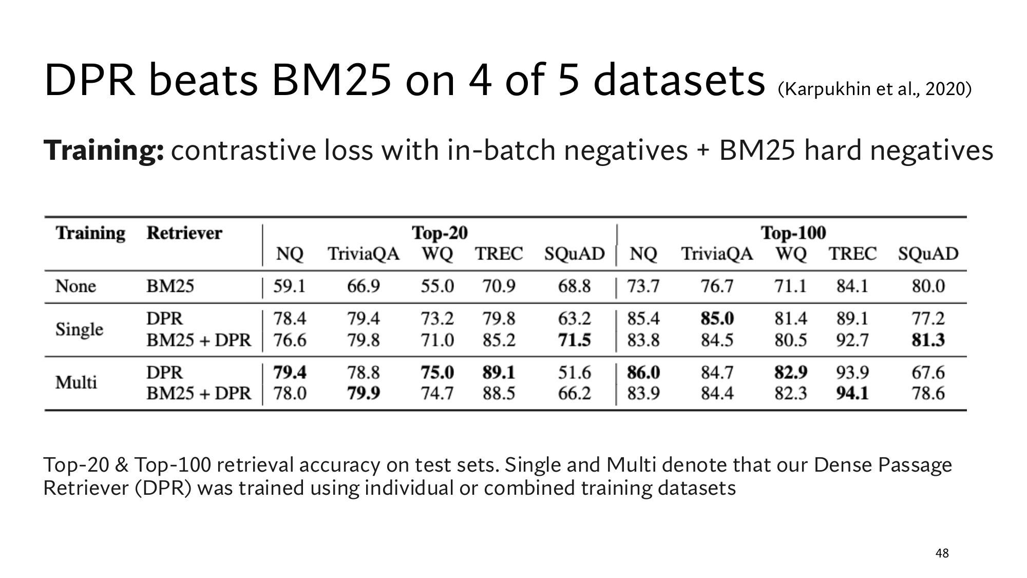
Real data shows the same thing. In lesson 12, top-20 accuracy on SQuAD was 68.8% for BM25 and 63.2% for DPR. On the same Stanford slide, a retriever that combines the two reaches 71.5%, ahead of both.
Think first
The query is refund policy for order #A77-310. Which part will BM25 catch, and which part will the dense retriever catch?
Show the answer
BM25 catches the rare literal A77-310 exactly. The dense retriever can match refund policy to a passage about money back rules, which shares no word with it.
2Hybrid search, and simply adding the scores
Hybrid search runs both retrievers and merges their two ranked lists into one list.Lesson 6 called merging lists . The simplest way is to add each passage's two scores: the BM25 score and the dense retriever's . my scores
Think first
The BM25 scores of E1, E3 and E2 are 7.2, 3.1 and 1.0, and their cosines are 0.79, 0.75 and 0.82. If you add the two, where does E2, the dense retriever's first passage, end up?
Show the answer
At rank 3, the bottom. The table below has the arithmetic.
Passage
BM25 score
Cosine
Plain sum
E1
7.2
0.79
7.99
E3 (wrong)
3.1
0.75
3.85
E2
1.0
0.82
1.82
After adding, the order is E1, E3, E2, exactly BM25's order. The reason is the scale of the two scores. The cosines spread from 0.75 to 0.82, only 0.07, while BM25 spreads from 1.0 to 7.2, which is 6.2.
BM25's spread is about 90 times the cosine's, so in the sum the cosine has almost no effect. A cosine always stays between −1 and 1, while BM25 has no upper limit. You could divide BM25 by some number, but that number would differ for every corpus, and you would have to find it each time.
3Reciprocal rank fusion: merging ranks instead of scores
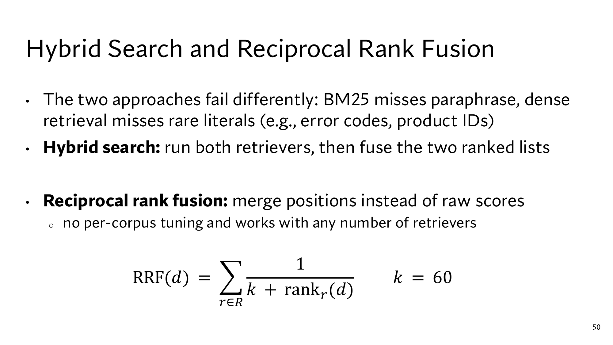
The scores have different scales, but ranks have the same scale in every retriever: first, second, third. Reciprocal rank fusion, or RRF, turns a passage's rank in each list into 1 ÷ (60 + rank), and adds these numbers over all lists. The passages are then ordered by this sum.
E1 is at rank 1 in BM25's list, so it gets 1 ÷ (60 + 1) = 1 ÷ 61 = 0.01639, about 0.0164. In the dense list it is at rank 2, so it gets 1 ÷ 62 = 0.01613. E1's RRF is the sum: 0.01639 + 0.01613 = 0.03252.
Passage
From BM25
From dense
Sum
E1
1 ÷ (60 + 1) = 0.01639
1 ÷ (60 + 2) = 0.01613
0.03252
E2
1 ÷ (60 + 3) = 0.01587
1 ÷ (60 + 1) = 0.01639
0.03227
E3 (wrong)
1 ÷ (60 + 2) = 0.01613
1 ÷ (60 + 3) = 0.01587
0.03200
The new order is E1, E2, E3. Both correct passages moved to the top, and E3 dropped to the bottom, because it was not first in any list.
The three sums sit close together, and the reason is how a fraction behaves. When the bottom of 1 ÷ (60 + rank) grows, the fraction shrinks. But going from 61 to 62 makes the bottom only 1.6% bigger, so the fraction also shrinks by only about 1.6%. That is why RRF numbers stay close together, and only their order matters.
Stanford's slide writes the same arithmetic as a formula:
RRF(d) = ∑r ∈ R1k + rankr(d), k = 60
d
A passage, such as E1.
R
The set of retrievers, here {BM25, dense}. The r ∈ R under the means: add over every retriever r in R.
rankr(d)
The rank of d in retriever r's list. For E1, 1 in BM25 and 2 in dense. A list that does not contain d adds nothing.
k
A fixed number, 60. It is not the k of top-k.
Stanford's slide: Hybrid Search and Reciprocal Rank Fusion. The first line is step 1, the second is step 2, and at the bottom is the RRF formula. The small line says RRF needs no per-corpus tuning and works with any number of retrievers. Click the image to open it at full size.
What k = 60 does
k = 60 shrinks the gap between rank 1 and rank 2, so rank 1 in a single list cannot decide the result on its own. With k = 0, rank 1 would get 1 and rank 2 would get 0.5, half as much. With k = 60, they get 0.01639 and 0.01613.
Suppose passage A is only in BM25's list, at rank 1, and passage B is at rank 3 in both lists: my example
With k = 0, A gets 1 ÷ 1 = 1, and B gets 1 ÷ 3 + 1 ÷ 3 = 0.667. A wins.
With k = 60, A gets 1 ÷ 61 = 0.0164, and B gets 1 ÷ 63 + 1 ÷ 63 = 0.0317. B wins.
So with k = 60, the winner is the passage that both retrievers place near the top.
Change k yourself
A is at rank 1 in one list, and B is at rank r in both lists. Change k and r and see how long B stays ahead.
Passage
Arithmetic
RRF
Think first
In lesson 6, the original query's list was: queue log, forum post, office hours page. The rewritten query's list was: office hours page, queue log. What order does RRF give?
Show the answer
Queue log: 1 ÷ 61 + 1 ÷ 62 = 0.03252. Office hours page: 1 ÷ 63 + 1 ÷ 61 = 0.03227. The forum post is only in the first list: 1 ÷ 62 = 0.01613. The order is queue log, office hours page, forum post.
The price of RRF is that it forgets how strong a score was. Whether E1's BM25 score is 7.2 or 70, rank 1 gives 1 ÷ 61 both times.
4Cross-encoder: reading the query and the passage together
E1 and E2 are at the top of the RRF list only because the two retrievers agreed on them. Neither retriever read the query and the passage together. In a , a passage's vector is made before any question arrives, and the two meet only at the final dot product.
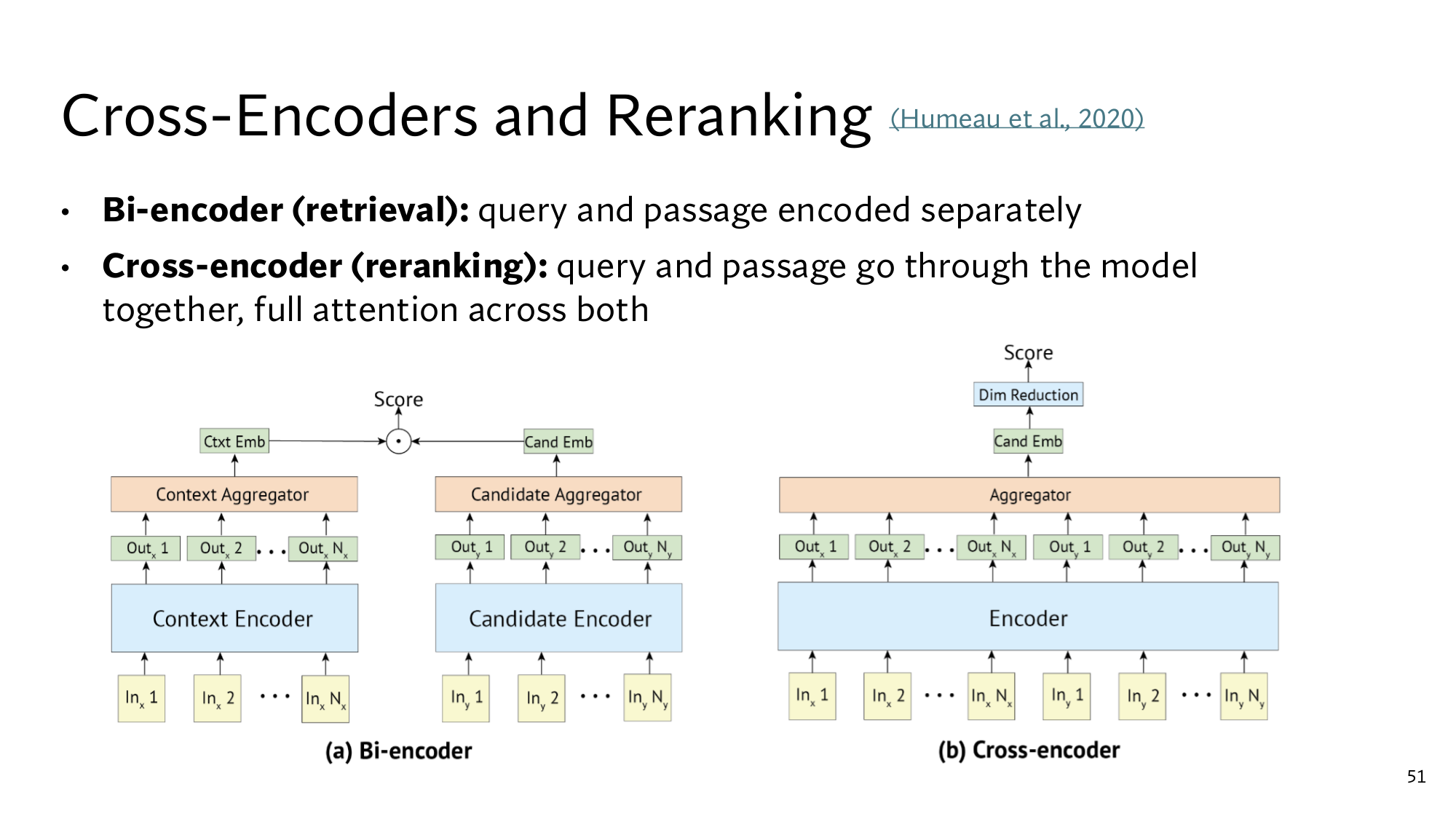
A cross-encoder joins the query and the passage into one text, feeds it to one model, and gets a single score for that pair. The model is usually an encoder such as .
Attention: each token updates its vector from the other tokens
An encoder makes a vector for every and then updates it many times. In attention, each token takes a weighted average of the other tokens' vectors and uses it as its new vector. In a weighted average you multiply each vector by its weight and add them up, and the weights add up to 1.
In a cross-encoder, the query's tokens can also look at the passage's tokens, which Stanford's slide calls full attention across both. Below, every vector has 2 numbers: the first says how much the token leans toward counted data, and the second how much it leans toward opinion. my numbers
The query token crowded starts as [0.5, 0.5]. When the query is joined with the queue log, crowded gives weight 0.6 to the queue log's averaged [1.0, 0.0] and 0.4 to itself:
With the forum post, the same 0.6 goes to usually [0.0, 1.0], and crowded becomes [0.2, 0.8]. So the same query token gets a different vector with every passage. In a bi-encoder, attention runs only inside the query, so crowded keeps one vector for every passage.
At the end, the model gathers the whole pair into one vector and turns it into a score. The reranker in lesson 6 gave the queue log 0.92, the office hours page 0.41 and the forum post 0.35 on the least-crowded question. The retriever had given the queue log and the forum post the same 2. my scores from lesson 6
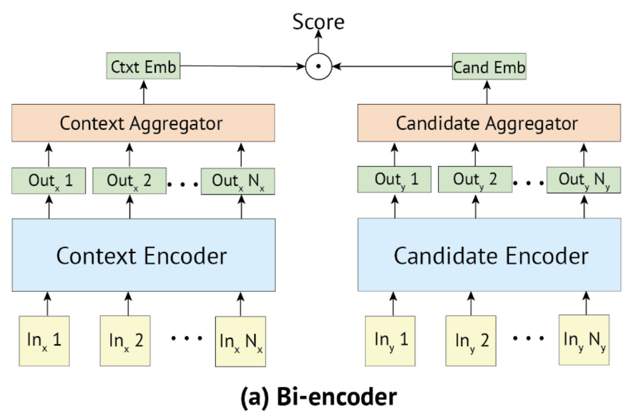
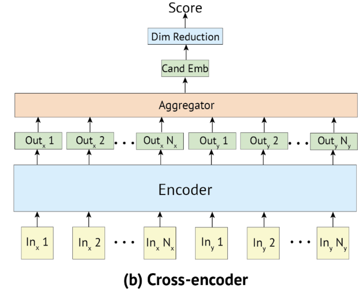
Stanford's slide: Cross-Encoders and Reranking. On the left, in the bi-encoder, the query (Inx) and the passage (Iny) go through separate encoders. On the right, in the cross-encoder, both go through one Encoder together.
The price: nothing can be built in advance
Every vector in a cross-encoder depends on the query, so nothing about a passage can be computed before the question arrives. On every query it has to run the whole model once for every passage, while a bi-encoder ran the model once per query.
According to Stanford's slide, a cross-encoder built on BERT-base takes 10,700 ms for 1,000 passages, which is 10.7 ms per passage. BERT-base is the smaller version of BERT. For the 60,000 passages of the company in lesson 2, one query would take 60,000 × 10.7 ms = 642 seconds, about 11 minutes.
5Reranking a shortlist
A retriever is fast but looks at passages roughly, and a cross-encoder is accurate but slow. So a fast retriever first picks the top few passages, such as the top 100, and then the cross-encoder scores and sorts only those again. This short list is called the shortlist, and the second step is reranking.
Step
On what
Time
1. BM25 and dense, then RRF
The whole corpus
BM25 62 msdense tens of ms, from Stanford's slide
2. Reranking with the cross-encoder
Top-100 shortlist
100 × 10.7 = 1,070 ms
3. Into the LLM's prompt
Top 5 after reranking
–
The whole corpus would take 642 seconds, and the shortlist takes about 1 second. A Stanford table shows the gain in accuracy. Its data is MS MARCO: real Bing search questions and about 8.8 million passages. MS MARCO description from the paper
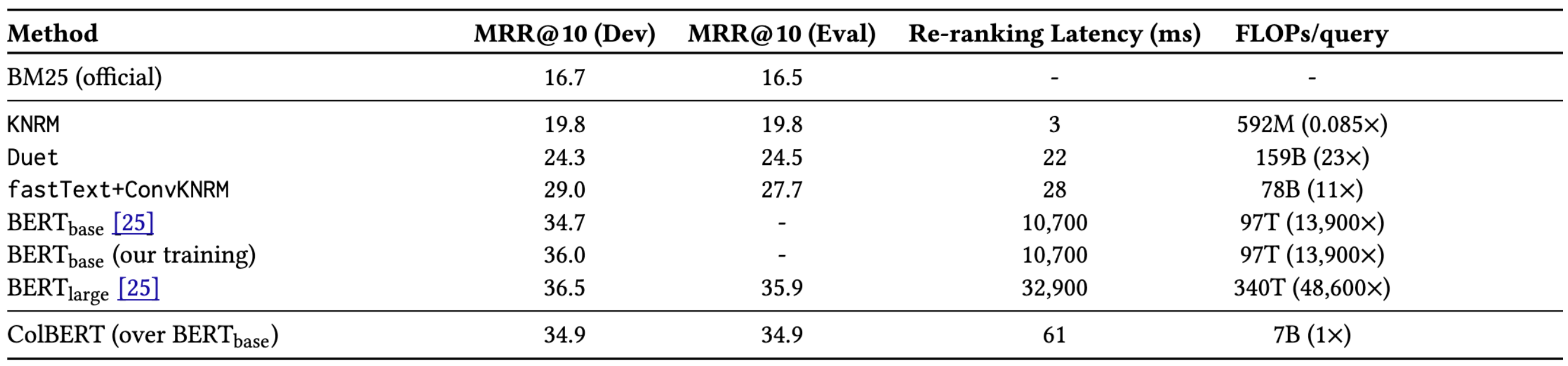
There, BM25 alone gets an of 16.7. In lesson 13 this was one over the rank of the first correct passage, such as 0.5 at rank 2. The table writes it multiplied by 100. Rerank BM25's top 1,000 with a BERT-base cross-encoder, and MRR@10 becomes 34.7. So reranking roughly doubles MRR@10: 34.7 ÷ 16.7 = 2.08.BM25's top 1,000 from the paper
A reranker has a limit: it only changes the order of the shortlist, and it cannot bring in a passage that is not there. This is the from lesson 2. If the shortlist holds the right passage for 60 out of 100 questions, the reranker cannot go above 60 either.
So the first step needs high recall, and hybrid search provides it: both E1 and E2 reach the shortlist.
Think first
Each query has a budget of 500 ms. The retriever takes 50 ms, and the cross-encoder takes 10.7 ms per passage. At most how many passages can the shortlist hold?
Show the answer
That leaves 500 − 50 = 450 ms for reranking. 450 ÷ 10.7 = 42.06, so 42 passages.
From here: the Stanford level
The steps above are the same as in the easy version. The steps below take you to the level of the Stanford slides: first the maths of RRF and the experiment behind k, then another way to put scores on one scale. After that comes the cross-encoder from inside, then the full cost, and finally you read the slides yourself. Every piece of maths is explained where it first appears.
6The maths of RRF: how k shrinks the gap between ranks
All of RRF's behaviour comes from one fraction: 1 ÷ (k + rank). Step 3 used k = 60. The table below shows how the same fraction changes for different k: my arithmetic
Rank
k = 0
k = 10
k = 60
1
1
0.09091
0.01639
2
0.5
0.08333
0.01613
3
0.333
0.07692
0.01587
10
0.1
0.05000
0.01429
100
0.01
0.00909
0.00625
Rank 1 ÷ rank 2
2
1.09
1.016
With k = 0, rank 1 is twice rank 2 and a hundred times rank 100. With k = 60, rank 1 is only 1.016 times rank 2, and 2.6 times rank 100. The reason is that with k = 60 the bottom of the fraction already holds 60. Adding 1 to the rank then takes the bottom from 61 to 62, a change of 1.6%, while with k = 0 the same step takes 1 to 2, a change of 100%.
Rank r in both lists against rank 1 in one list
Now look at A and B from step 3 for any k and r. A is at rank 1 in one list only, so it gets 1 ÷ (k + 1). B is at rank r in both lists, so it gets 2 ÷ (k + r).
There is a simple rule for comparing two positive fractions: a ÷ b is bigger than c ÷ d exactly when a × d is bigger than c × b. For example, 2 ÷ 3 is bigger than 1 ÷ 2, because 2 × 2 = 4 and 1 × 3 = 3. The same rule gives B's condition in three steps:
2 ÷ (k + r) is bigger than 1 ÷ (k + 1) exactly when 2 × (k + 1) is bigger than 1 × (k + r).
That is, when 2k + 2 is bigger than k + r.
Subtract k from both sides: when k + 2 is bigger than r.
B stays ahead as long as r is smaller than k + 2. With k = 60, B stays ahead up to rank 61. Check: 2 ÷ 121 = 0.016529, which is bigger than 1 ÷ 61 = 0.016393. At r = 62 the two are tied, because 2 ÷ 122 = 1 ÷ 61. With k = 0, B is ahead only at r = 1.
So k decides how deep the agreement between the two retrievers counts. With k = 60, agreement anywhere inside the top 61 outweighs rank 1 in a single list. The widget in step 3 shows the same rule: it keeps B ahead up to r = k + 1.
k is a hyperparameter, and the RRF paper's experiment
Training does not learn k. Someone has to choose it in advance. Lesson 11 called such a number a , like BM25's k1 and b, which the DPR paper set to 0.9 and 0.4.
k = 60 comes from the 2009 paper by Cormack, Clarke and Büttcher that introduced RRF. According to the paper, k = 60 was fixed in a small early experiment and never changed afterwards. In that experiment the paper fused the lists of 30 search systems and measured the result for each k with MAP. from the paper
MAP, or mean average precision, is a number between 0 and 1 for the quality of a ranking, and the bigger it is, the better the ranking. It averages the at the rank of each correct document. In lesson 6, precision was the share of returned passages that are right, such as 0.5 when 1 of 2 is right.
k in RRF
MAP
0
.2072
10
.2123
60
.2145
80, the best
.2147
500
.2098
Best single system, no fusion
.2016
Fusion of 30 systems on TREC topics 351 to 400. from the paper
Going from k = 0 to 60 raises MAP from .2072 to .2145, and at 500 it falls back to .2098. Every k from 30 to 100 gives a MAP between .2138 and .2147. In the paper's words, k = 60 was near-optimal, but the choice was not critical. At every k, RRF beats the best single system's .2016.
The paper also explains the reasoning behind k. Top ranks matter more, but the effect of lower ranks should not vanish, as it would with an exponential formula. With a score of 1 ÷ 2rank, for example, rank 10 would get 1 ÷ 1,024, about 0.001. In RRF with k = 60, rank 10 gets 87% of what rank 1 gets. According to the paper, k also damps the high ranking that a single outlier system gives, which is exactly what happened with A and B. from the paper
7Putting scores on one scale: min-max, and the DPR paper's sum
In step 2 the plain sum of scores failed because the two scores had different scales. RRF dropped the scores. The other route is to bring both scores onto one scale first, and then add them.
Min-max normalisation maps each list's scores onto 0 to 1: the smallest score becomes 0, the largest becomes 1, and the rest fall in between in proportion. The formula is (x − min) ÷ (max − min). In BM25's list the min is 1.0 and the max is 7.2, so E3's 3.1 becomes (3.1 − 1.0) ÷ (7.2 − 1.0) = 2.1 ÷ 6.2 = 0.339. For the cosines the min is 0.75 and the max is 0.82, so E1's 0.79 becomes 0.04 ÷ 0.07 = 0.571. my scores from step 2
Passage
BM25 on 0 to 1
Cosine on 0 to 1
Sum
E1
1from 7.2
0.571from 0.79
1.571
E2
0from 1.0
1from 0.82
1.000
E3 (wrong)
0.339from 3.1
0from 0.75
0.339
Now the order is E1, E2, E3, the same as RRF. In this example, min-max fixed the scale problem.
The weakness of min-max: the result depends on the list's min and max
Every min-max score depends on the list's min and max, and those depend on which passages made it into the list. Suppose a fourth, weak passage E4 with cosine 0.60 also enters the dense list. Now the cosine min is 0.60, and the spread is 0.82 − 0.60 = 0.22: my example
E1: (0.79 − 0.60) ÷ 0.22 = 0.19 ÷ 0.22 = 0.864, and the sum is 1 + 0.864 = 1.864.
E3: (0.75 − 0.60) ÷ 0.22 = 0.15 ÷ 0.22 = 0.682, and the sum is 0.339 + 0.682 = 1.021.
E2: (0.82 − 0.60) ÷ 0.22 = 1, and the sum is 0 + 1 = 1.000.
The wrong E3 is now above the correct E2, although the scores of E1, E2 and E3 did not change at all. One low passage joining the list was enough to flip the order. In RRF, E4 would enter the dense list at rank 4, the ranks of E1, E2 and E3 would stay the same, and so would their RRF values.
The DPR paper's BM25 + DPR: a sum of scores with λ
In the dense version of lesson 12, the DPR paper's table had a column called BM25 + DPR. The paper builds this column by adding scores, not with RRF. It takes the top 2,000 passages from BM25 and from DPR, and sorts all passages from both lists again with this score: from the paper
BM25(q, p) + λ · sim(q, p), λ = 1.1
Here sim(q, p) is DPR's dot-product score, and λ (lambda) is a number that multiplies it. The paper chose λ = 1.1 by checking accuracy on the dev set, the questions researchers use to check their decisions. So this is step 2's multiplying by a number, and that number had to be chosen by looking at data.
The right λ depends on the scale of the scores. On our cosines, λ = 1.1 changes nothing: E1 gets 7.2 + 1.1 × 0.79 = 8.069, E3 gets 3.925, E2 gets 1.902, and the order is BM25's again. DPR's sim is a dot product, not a cosine, and it has no upper limit.
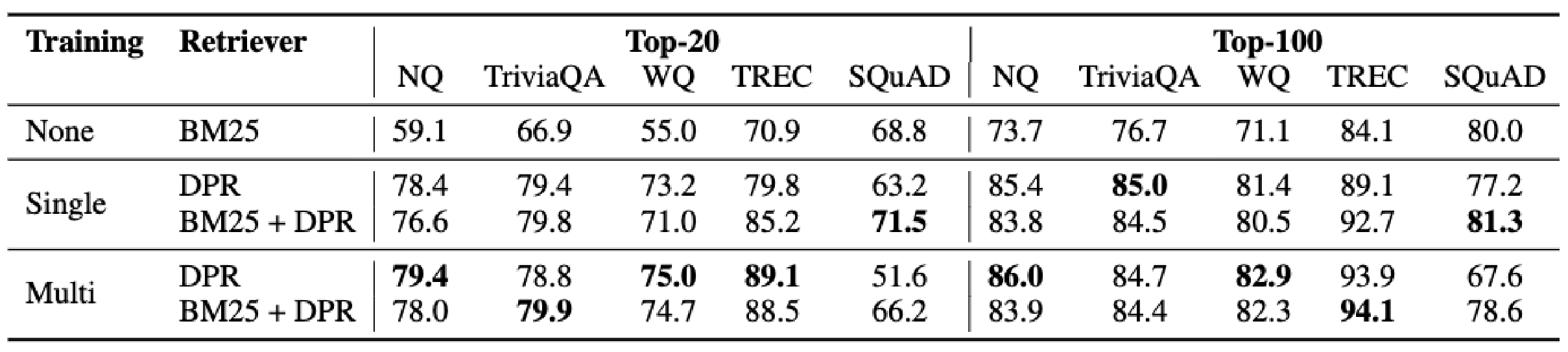
Stanford's results slide shows the same column. Single means that DPR was trained separately on each dataset:
Dataset
BM25
DPR
BM25 + DPR
NQ
59.1
78.4
76.61.8 below DPR
TriviaQA
66.9
79.4
79.80.4 above
WQ
55.0
73.2
71.02.2 below DPR
TREC
70.9
79.8
85.25.4 above
SQuAD
68.8
63.2
71.52.7 above BM25
Top-20 accuracy (%) on the test sets. “Above” and “below” compare with the better of the two retrievers.
On TREC, SQuAD and TriviaQA the sum beats both retrievers. On NQ and WQ it falls behind DPR, and on exactly these two BM25 was 19.3 and 18.2 points behind DPR. The table shows that merging pays off when both retrievers are good in their own way, and that one much weaker retriever can drag the merged list down.
8The cross-encoder from inside: attention weights, the score and training
Attention weights come from a softmax
In step 4, crowded gave weight 0.6 to averaged and 0.4 to itself. The model works these weights out itself. For every pair of tokens it first computes a score, and then a turns those scores into weights. In lesson 4, softmax meant taking escore for each score and dividing by the sum, so that the results add up to 1.
Suppose the pair crowded and averaged has score 0.9, and crowded with itself has score 0.5: my numbers
e0.9 = 2.46 and e0.5 = 1.65. Their sum is 4.11.
Weight of averaged: 2.46 ÷ 4.11 = 0.599, about 0.6.
Weight of crowded itself: 1.65 ÷ 4.11 = 0.401, about 0.4.
This score is really a of two vectors, but not of the tokens' own vectors. The model transforms each token's vector with numbers it has learned to make new vectors, and takes their dot product. Training adjusts exactly these numbers, so that a pair of tokens that matter to each other gets a large score.
The input layout, and one vector to one score
The 2019 paper by Nogueira and Cho turns BERT into a reranker in exactly this way, and the BERT-base 34.7 in Stanford's table comes from this method. The input is a single text: first a special token [CLS], then the query, then a special token [SEP], then the passage, and finally another [SEP]. [SEP] only separates the two parts. The query has at most 64 tokens, and the whole input at most 512. from the paper
The [CLS] vector is also built by attention, and it takes a weighted average over the tokens of both the query and the passage. That is why, at the end, this single vector carries the whole pair. The Aggregator box in the slide's diagram does exactly this: it takes one vector out of all the output vectors, and in Humeau's paper it is the first one. from the paper
Then a small layer turns this vector into one number. In Humeau's paper this layer is a dot product with a vector W that training learns. from the paper This is the Dim Reduction box in the diagram, because it shrinks the whole vector down to one number. Suppose the queue log pair's vector is [0.8, 0.2] and W = [2.0, −1.0]: my numbers
Forum post, whose vector is [0.2, 0.8]: 0.2 × 2.0 + 0.8 × (−1.0) = 0.4 − 0.8 = −0.4.
From score to probability, and the training loss
Nogueira and Cho's reranker gives, instead of a raw score, the probability that the passage is relevant. from the paper A two-class layer like this gives two numbers, one for relevant and one for not relevant, and a softmax turns them into probabilities. Lesson 12 showed that adding the same number to all scores does not change a softmax. So only the difference between the two numbers matters, and the not-relevant number can be set to 0:
The queue log's relevant number is 2.44. e2.44 = 11.47, and e0 = 1.
The forum post's number is −0.62: e−0.62 = 0.54, and 0.54 ÷ 1.54 = 0.35.
The office hours page's −0.36 gives 0.41 the same way. These are lesson 6's three scores: 0.92, 0.41 and 0.35. 2.44, −0.36 and −0.62 are my numbers
In training, each question comes with its relevant passages and with non-relevant passages from BM25's top 1,000. The loss is the −ln from lesson 4: −ln(probability) for a relevant passage, and −ln(1 − probability) for a non-relevant one, because its correct answer is not relevant. from the paper
𝓛 = − ∑j ∈ Jpos ln sj − ∑j ∈ Jneg ln(1 − sj)
Jpos is the list of relevant passages, Jneg the list of non-relevant ones, and sj is passage j's probability. The paper writes log, meaning ln. On our two passages:
The queue log is relevant, with s = 0.92: −ln 0.92 = 0.083.
The forum post is not relevant, with s = 0.35: −ln(1 − 0.35) = −ln 0.65 = 0.431.
The sum: 0.083 + 0.431 = 0.514.
The forum post's loss is larger because the model still gives it 0.35, and training pushes its score further down. The paper trained BERT-large with batch size 128 for 100,000 steps, that is, on 12.8 million question-passage pairs, which took about 30 hours. from the paper
Humeau's paper points out one more training difference: a cross-encoder cannot use the of lesson 12. In a bi-encoder, each passage in the batch is encoded once, and every question can use it as a negative. In a cross-encoder, the model runs separately for every question-passage pair. So the paper uses separately supplied negatives, and keeps the batch small because of the extra memory. from the paper
9The cost: running the model N times against once
Counting makes the difference between a cross-encoder and a bi-encoder clear. Suppose the corpus has N passages and Q questions arrive per day:
Work
Bi-encoder
Cross-encoder
Before any question
The passage encoder N times, only once
Nothing
On each question
The question encoder once, and N dot products
The whole model N times
N = 60,000 and Q = 10,000
60,000 + 10,000 = 70,000 model runs
10,000 × 60,000 = 600 million model runs
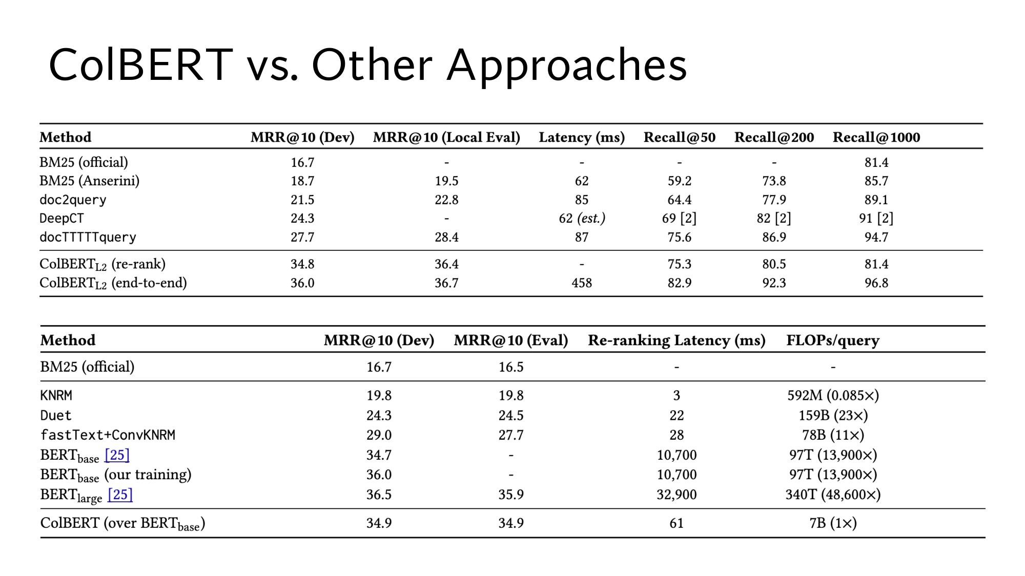
How expensive one model run is shows up in the lower table of Stanford's ColBERT slide. Its last column gives per query, the number of multiplications and additions. Reranking 1,000 passages with the BERT-base cross-encoder takes 97T FLOPs:
T stands for trillion, 1012. Per passage that is 97T ÷ 1,000 = 97 billion FLOPs.
A dot product of two 768-number vectors takes 768 multiplications and 768 additions, which is 1,536 FLOPs.
97 billion ÷ 1,536 = about 63 million. So one cross-encoder run costs about as much as 63 million dot products.
Humeau's paper timed both methods on the same GPU, on a dialogue task: from the paper
Candidates
Bi-encoder
Cross-encoder
1,000
19 ms
2,600 ms
100,000
22 ms
266,000 msestimated, not measured
At 1,000 candidates the cross-encoder is 2,600 ÷ 19 = about 137 times slower. At 100,000 the bi-encoder's time hardly changes, because the candidate vectors already exist and only the dot products grow. The cross-encoder's time grows in step with the number of candidates. This hardware differs from the hardware behind Stanford's slide, so do not compare these ms with the 10,700 ms.
A bigger model is more accurate but slower still. In Stanford's table, BERT-large reaches an MRR@10 of 36.5, 1.8 above BERT-base. But it takes 32,900 ms for 1,000 passages, 3.07 times as long. Within the 450 ms from step 5, BERT-large could rerank only 450 ÷ 32.9 = 13 passages, against 42 for BERT-base.
The recall ceiling in real numbers
In the upper table of the same slide, BM25's Recall@1000 on MS MARCO is 81.4. comes from lesson 13: the correct passages found in the top k divided by all correct passages, such as 0.5 when 1 of 2 is found. In MS MARCO each question has on average one correct passage. from the paper So 81.4 roughly means that for 81.4 out of 100 questions the correct passage is in BM25's top 1,000, and for 18.6 it is not.
BERT-base reranked exactly these 1,000 BM25 passages, so its Recall@1000 cannot go above 81.4 either. The table's ColBERTL2 (re-rank) row shows this: it also reranks BM25's top 1,000, and its Recall@1000 is exactly 81.4. Reranking took MRR@10 from 16.7 to 34.7, but BM25 fixed the recall ceiling at 81.4.
Hybrid search raises this ceiling, because the merged lists of two retrievers give the correct passage more chances to appear than one list does. Lesson 15 calls this design, a fast step first and an expensive step after it, a . There, ColBERT searches the whole corpus and lifts Recall@1000 to 96.8.
10Now read Stanford's slides yourself
Below are five Stanford slides, unchanged, each followed by its key part enlarged. Under each slide are a few questions. Think of the answer first, then open it. If something stops you, go back to the step named in the answer. If a slide looks small on a phone, click the image.
Stanford's hybrid search slide, and below it the first point and the formula, enlarged.
Read the hybrid search slide
The first point says BM25 misses paraphrase and dense retrieval misses rare literals. Which of E1, E2 and E3 are examples of each?
Show the answer
E2 is the paraphrase, and BM25 put it at rank 3. E1's E-4012 is the literal, and dense retrieval put E1 at rank 2, while BM25 put it at rank 1. (Step 1)
In the formula, k = 60 is added to rankr(d). With k = 60, which passages beat a passage at rank 1 in one list?
Show the answer
Every passage at rank 61 or better in both lists, because a passage in both lists is ahead while r is smaller than k + 2. (Steps 3 and 6)
The slide says no per-corpus tuning. Why does the DPR paper's BM25 + DPR not meet this?
Show the answer
It uses λ = 1.1, which the paper chose on the dev set. RRF needs no number chosen by looking at data, because ranks have the same scale in every corpus. (Steps 2 and 7)
Stanford's cross-encoder slide, and below it both diagrams, enlarged. Inx are the query's tokens, and Iny the passage's.
Read the cross-encoder slide
In the bi-encoder, there is a ⊙ under Score. What does it do, and why is it missing from the cross-encoder?
Show the answer
⊙ is the dot product of Ctxt Emb and Cand Emb, the score from lesson 12. In the cross-encoder both texts are in one Encoder, so there are no two separate vectors. There, Dim Reduction turns one vector straight into a number. (Steps 4 and 8)
In the cross-encoder, only Cand Emb sits above the Aggregator, and there is no Ctxt Emb. Why?
Show the answer
A cross-encoder never builds a separate vector for the query. The one vector the Aggregator gives belongs to the whole pair, and in Humeau's paper it is the first token's output, like [CLS]. (Step 8)
In the bi-encoder you can build Cand Emb in advance and keep it in an index. Why can a cross-encoder not do this?
Show the answer
Because the Outy vectors are also built by looking at the query's tokens, just as crowded's vector differed with every passage. Change the query, and everything changes. (Step 4)
Stanford's DPR results slide, and below it the table, enlarged. Lesson 12 read the BM25 and DPR rows. Here, read the BM25 + DPR rows.
Read the BM25 + DPR rows of the results slide
At top-20, on which datasets is the Single BM25 + DPR row below DPR?
Show the answer
On NQ (76.6 against 78.4) and on WQ (71.0 against 73.2). On both, BM25 was far behind: 59.1 and 55.0. (Step 7)
On SQuAD, BM25 + DPR is at 71.5. How far ahead of BM25 and DPR is that?
Show the answer
2.7 ahead of BM25's 68.8, and 8.3 ahead of DPR's 63.2. On SQuAD, BM25 alone was ahead of DPR, yet the merge got ahead of both. (Steps 1 and 7)
Are the BM25 + DPR rows built with RRF?
Show the answer
No. The DPR paper added scores with BM25(q, p) + 1.1 · sim(q, p) over the union of the two top-2,000 lists. from the paper (Step 7)
Stanford's ColBERT slide. First the lower, reranking table enlarged, then the upper table with recall. The ColBERT rows come in lesson 15. Dev and Eval are two separate question sets of MS MARCO.
Read the reranking rows of the ColBERT slide
In the lower table, BERTbase [25] has an MRR@10 of 34.7. What is [25], and which list does this reranker rerank?
Show the answer
[25] is the paper by Nogueira and Cho. Its reranker reranks BM25's top 1,000, and BM25 alone is at 16.7. from the paper (Steps 5 and 8)
Under FLOPs/query, BERTbase has 97T (13,900×). How many FLOPs is that per passage, and what is the 13,900× compared with?
Show the answer
Per passage, 97T ÷ 1,000 = 97 billion. The 13,900× compares with ColBERT's 7B in the last row: 97T ÷ 7B = about 13,900. (Step 9)
In the upper table, why is the Recall@1000 of ColBERTL2 (re-rank) exactly BM25 (official)'s 81.4?
Show the answer
Because the re-rank model sorts BM25's own top 1,000 again. Reranking changes the order, not the list, so the recall ceiling stays BM25's. (Steps 5 and 9)
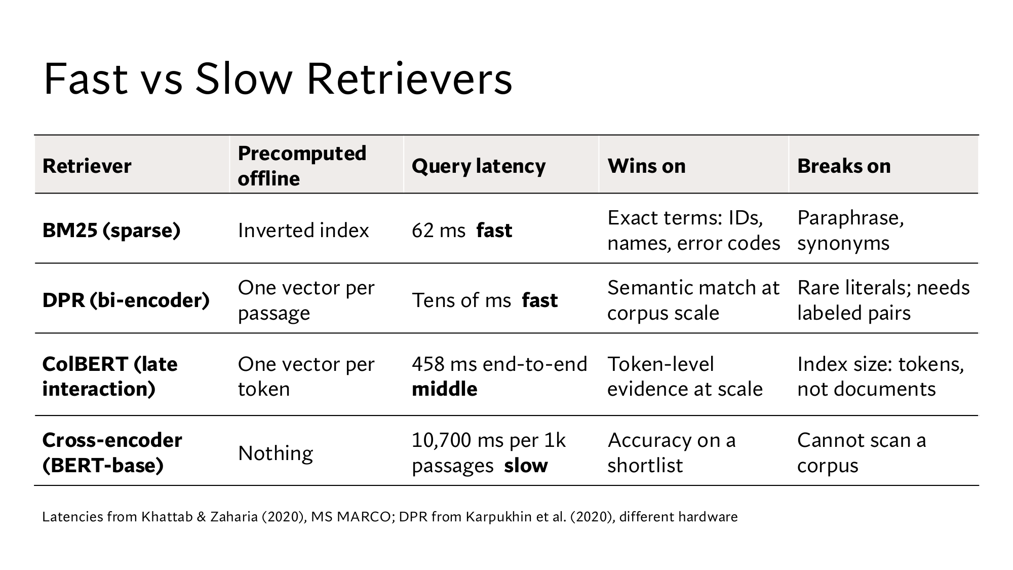
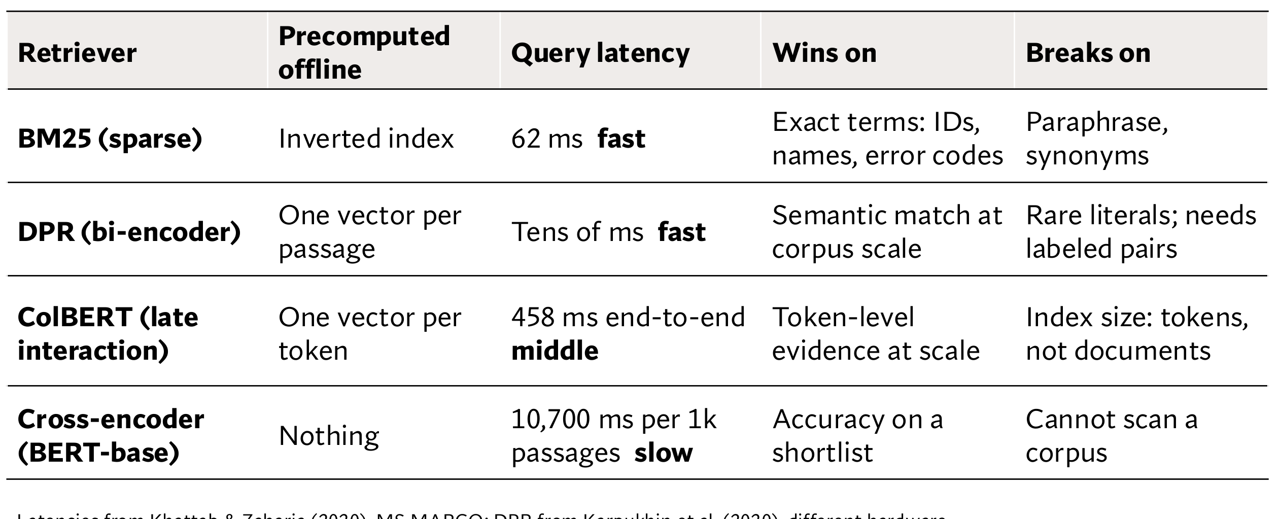
Stanford's comparison slide, and below it the table, enlarged. Lesson 12 read the BM25 and DPR rows. Here, read the cross-encoder row.
Read the cross-encoder row of the comparison slide
Why does the cross-encoder row say Nothing under Precomputed offline?
Show the answer
Because each of its vectors depends on the query, nothing about a passage can be built in advance. (Step 4)
Wins on says Accuracy on a shortlist, and Breaks on says Cannot scan a corpus. What do these mean in numbers for 60,000 passages?
Show the answer
The whole corpus would take 60,000 × 10.7 ms = 642 seconds per query, and a top-100 shortlist takes 1,070 ms. On a shortlist, reranking took MRR@10 from 16.7 to 34.7. (Steps 4 and 5)
3 points from this lesson
BM25 misses paraphrases, and a dense retriever misses rare literals. Hybrid search merges their lists, but the DPR paper's sum of scores fell behind DPR on NQ and WQ.
RRF adds 1 ÷ (k + rank) from each list. With k = 60, a passage at rank 61 or better in both lists beats rank 1 in a single list, because the condition is r < k + 2. The result of min-max depends on the list's min and max.
In a cross-encoder, attention runs between the query and the passage, so nothing can be built in advance, and one pair costs about as much as 63 million dot products. Reranking took MRR@10 from 16.7 to 34.7, but Recall@1000 stayed at BM25's 81.4.
New terms in this lesson
Paraphrase
The same statement in other words. For example, upload failed and upload keeps failing. BM25 misses it, because it counts shared words.
Literal
Text that has to match exactly, such as the error code E-4012 or the order ID A77-310. A dense retriever can miss it, and BM25 catches it as a rare word.
Hybrid search
Running both a word-based and a dense retriever and merging their lists. For example, making one list from BM25's E1, E3, E2 and dense retrieval's E2, E1, E3.
Reciprocal rank fusion (RRF)
1 ÷ (k + rank) from a passage's rank in each list, summed over all lists, with k = 60. For example, E1: 1 ÷ 61 + 1 ÷ 62 = 0.03252.
Attention
Each token takes a weighted average of the other tokens' vectors as its new vector, and the weights add up to 1. For example, if crowded [0.5, 0.5] gives weight 0.6 to averaged [1.0, 0.0], it becomes [0.8, 0.2].
Cross-encoder
A reranker that joins the query and the passage, feeds them to one model, and gets a direct score for the pair. It runs in full for every passage, for example 10.7 ms per passage with BERT-base.
Reranking
Scoring and sorting a fast retriever's shortlist again with an accurate model. For example, on MS MARCO, MRR@10 goes from 16.7 for BM25 alone to 34.7 after reranking with BERT-base.
Shortlist
The retriever's top few passages, on which the reranker runs. For example, the top 100 of 60,000 passages, which the cross-encoder handles in 1,070 ms.
Min-max normalisation
Mapping each list's scores onto 0 to 1 with (x − min) ÷ (max − min). For example, BM25's 7.2, 3.1 and 1.0 become 1, 0.339 and 0. The result depends on the list's min and max.
[CLS] and [SEP]
Special tokens in BERT's input. [CLS] comes first, and in a cross-encoder its last vector carries the whole pair. [SEP] separates the query from the passage, as in [CLS] query [SEP] passage [SEP].