Measuring a retriever: Hit@k, MRR, Recall@k and nDCG
Measuring a retriever means looking at its lists for a set of queries and counting how many right passages came back, and how high they sit. First someone has to write down the right passages for every query, and then each metric turns the lists into one number.
Lesson 2 counted recall roughly. Now run a retriever on the same 3 queries. For the first query the right passage comes back at rank 1, for the second at rank 2, and for the third not at all. In the top 3, the right passage arrived for 2 of the 3 queries, which is 0.667.
Then you improve the retriever, and the second query's right passage moves up to rank 1. If only one passage goes into the prompt, that query can now be answered too. Yet the top-3 count stays stuck at 0.667. This lesson builds numbers that can see that change.
The ladder for this lesson
The ladder has 10 steps. The first 5 are the same as in the easy version, and steps 6 to 10 take you to the level of the Stanford slides. Under each step you can see what you will be able to do after it.
What you need first: Lesson 2 (the 6 passages of the corpus, top-K, recall, the recall ceiling), Lesson 3 (the ∑ sign) and Lesson 4 (ln). From step 6 on, Lesson 8 (late chunking), Lesson 10 (ANN) and Lesson 12 (DPR, top-k accuracy) also help. If you already know a step, skip to the next one. A word with a dotted underline and ▾ opens its definition when you click it.
1Relevance labels and sets: write down the right passages first
Relevance labels are a list in which a person writes down, for each query, which passages are right. A retriever cannot tell you whether its own list is right, so before you can measure it, someone has to read the passages and make this list. Each passage can also get a grade: 3 means very useful, 1 means a little useful, and 0 means not useful.
The whole lesson uses the same 3 over lesson 2's corpus. Suppose a returns 5 passages for each query, with each passage's grade in brackets. my retriever and grades
Query
The retriever's order (grade)
Right passages
q1: Least crowded office hour?
queue log (3), old forum post (0), office hours page (1), syllabus (0), project page (0)
syllabus (0), Homework 1 announcement (0), project page (0), old forum post (0), queue log (0)
office hours page, grade 2
q1 has two right passages. The queue log has the crowd data, and the office hours page says that the Thursday 9am office hour is on Zoom. The real answer is in the queue log, so it gets grade 3, and the office hours page gets 1. q3's right passage is nowhere in the retriever's list.
Sets: short names for the right passages
The metric formulas give these lists short names, and for that they use sets. A set is a group of things written inside { }, and the order inside it does not matter.
The set of right passages for query q is written Rq, for example Rq1 = {queue log, office hours page}. The set of the retriever's top k passages is Topk(q). This k is the same as lesson 2's , only written small in formulas. So Top3(q1) = {queue log, old forum post, office hours page}. Three more signs come with sets:
∩ gives the things that are in both sets. Rq1 ∩ Top3(q1) = {queue log, office hours page}, so both of q1's right passages are in the top 3.
∅ is the empty set, with nothing in it. For q3, {office hours page} ∩ {syllabus, Homework 1 announcement, project page} has nothing in common, so it is ∅.
|A| is how many things set A holds. |Rq1| = 2, and for the set Q of all queries, |Q| = 3.
Labels have a cost. A person has to read and decide the right passages for every query, which is expensive. If that person misses a right passage, a retriever that finds it still loses on every metric.
2Hit@k and Failed@k: did a right passage arrive?
Hit@k checks, for each query, whether the top k holds at least one right passage, and then averages over the queries. If it does, the query gets 1, otherwise 0. At k = 3, q1's top 3 holds the queue log and the office hours page, so 1. q2's top 3 holds the syllabus, so 1. q3's top 3 holds no right passage, so 0.
Add the three queries' numbers: 1 + 1 + 0 = 2.
Divide by the number of queries, which gives the average: 2 ÷ 3 = 0.667.
Hit@3 = 0.667, the number from the start of the lesson.
This “1 if true, 0 if false” rule has its own sign: . For example, 𝟙[2 > 1] = 1 and 𝟙[2 > 3] = 0. In Hit@k the condition is that Rq ∩ Topk(q) is not empty, written ≠ ∅, where ≠ means “not equal to”. For q3 the intersection is empty, so 𝟙[Rq3 ∩ Top3(q3) ≠ ∅] = 0. The formula holds the two steps above:
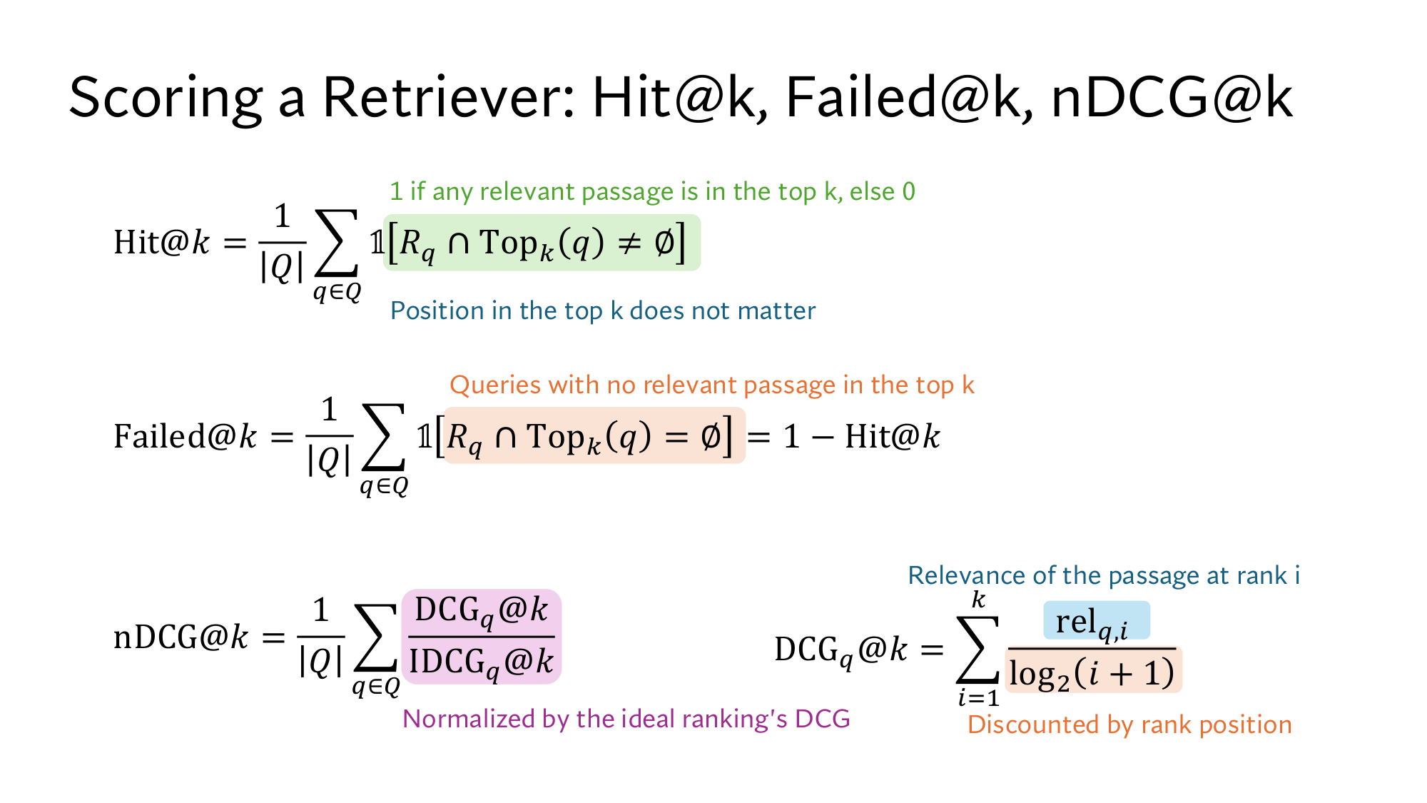
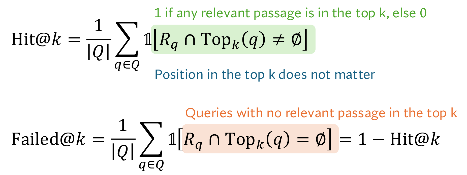
Hit@k = 1|Q|∑q ∈ Q 𝟙[Rq ∩ Topk(q) ≠ ∅]
q ∈ Q
Add over every query q in Q. ∈ means “one of the members of this set”. Here 1 + 1 + 0 = 2.
1 ÷ |Q|
Divide by the number of queries, which makes it an average. Here 2 ÷ 3 = 0.667.
Failed@k is the opposite: the share of queries where not a single right passage reached the top k. Each query scores 1 on either Hit or Failed, never both, so Failed@k = 1 − Hit@k. Here Failed@3 = 1 − 0.667 = 0.333, because 1 query out of 3, q3, failed.
Hit@3 = 0.667 is also lesson 2's here, because no more than 2 of the 3 queries can be answered from the passages. The same numbers come back later under other names. The of lesson 8 is Failed@20, because each query there had one right chunk. The of lesson 12 is Hit@20.
Now look at the improvement from the start. q2's syllabus moved from rank 2 to rank 1, but both times it is inside the top 3, so q2 gets 1 both times. Hit@k does not look at where inside the top k the right passage sits. Stanford's slide says so under Hit@k: Position in the top k does not matter.
Take k = 1 and the improvement shows: Hit@1 was 1 ÷ 3 = 0.333, and after the improvement it is 2 ÷ 3 = 0.667. But then Hit@1 cannot tell rank 2 from rank 5, because both get 0. So at any single k, Hit@k sees only one slice of the order.
3MRR@k: how high the first right passage is
The reciprocal rank is 1 divided by the rank of the first right passage, and MRR is its average over the queries. The reciprocal of a number is 1 divided by that number. If the first right passage is at rank 1, the reciprocal rank is 1 ÷ 1 = 1. At rank 2 it is 1 ÷ 2 = 0.5, and at rank 3 it is 1 ÷ 3 = 0.333. If no right passage is in the top k, it is 0.
Now look at the three queries at k = 3. q1's first right passage, the queue log, is at rank 1, so 1. q2's syllabus is at rank 2, so 0.5. q3 has no right passage in the top 3, so 0.
Add the three reciprocal ranks: 1 + 0.5 + 0 = 1.5.
Divide by 3 queries: 1.5 ÷ 3 = 0.5.
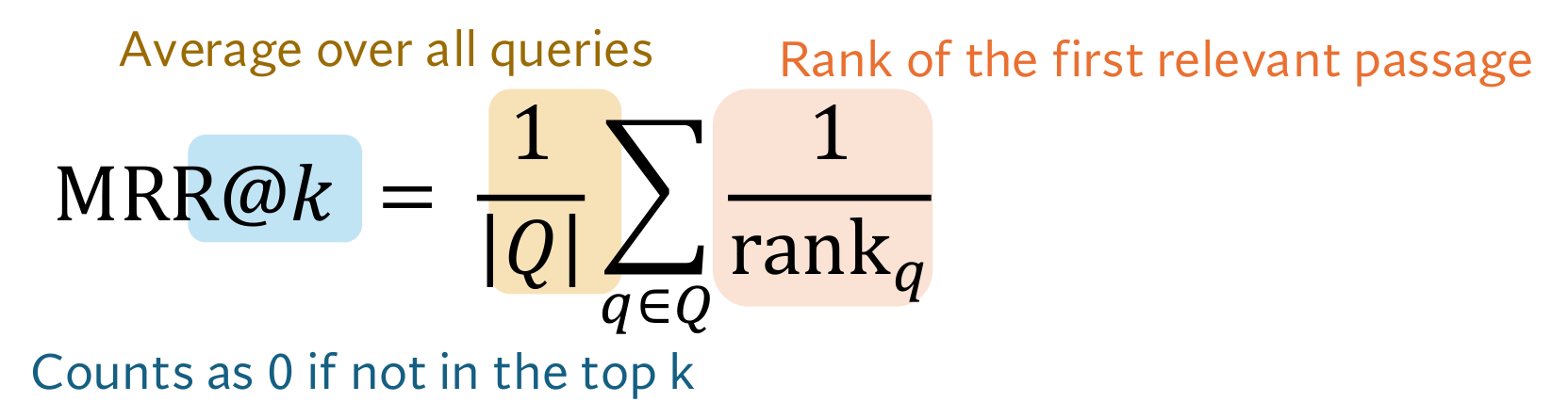
This average is called MRR, the mean reciprocal rank, and here MRR@3 = 0.5. The formula holds the same two steps:
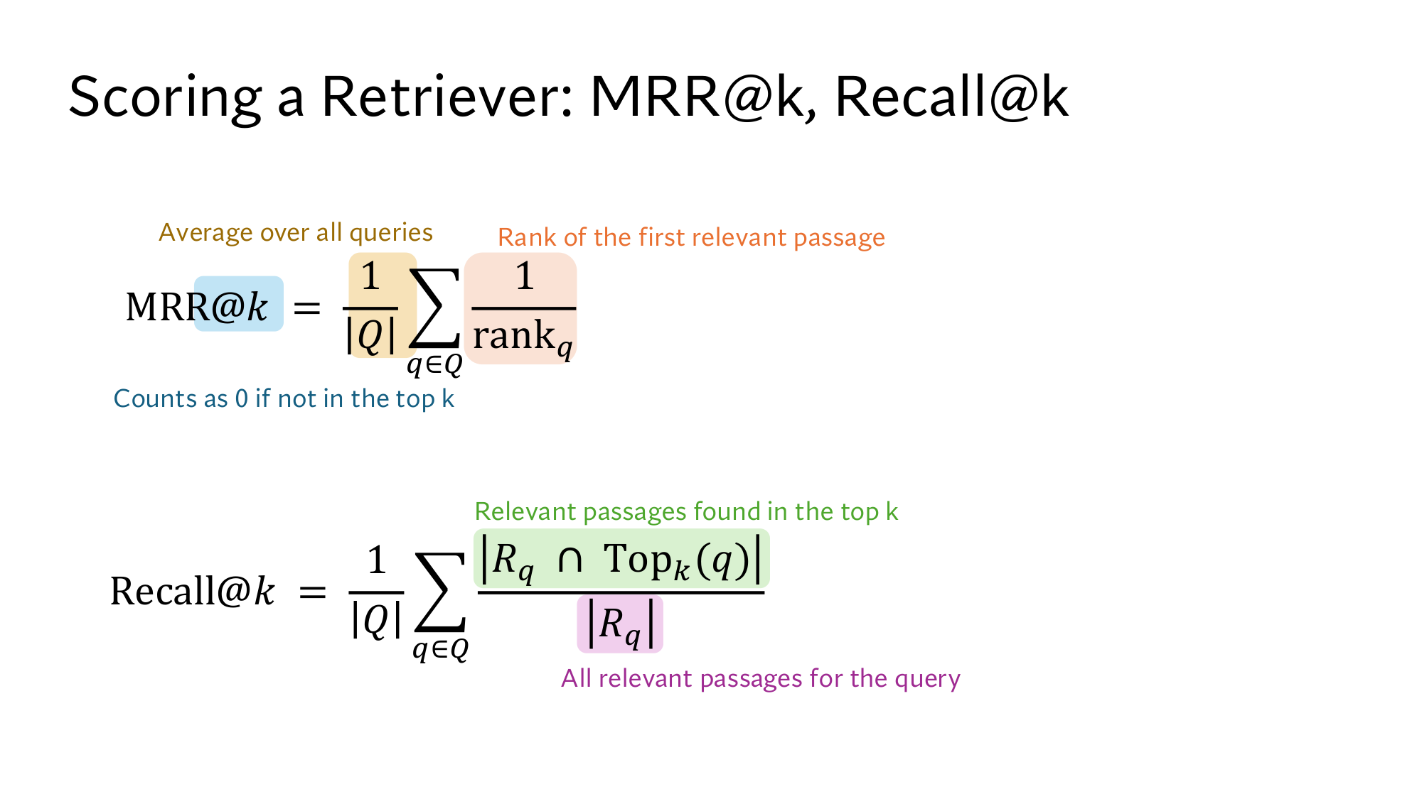
MRR@k = 1|Q|∑q ∈ Q1rankq
rankq
The rank of query q's first right passage: 1 for q1, and 2 for q2. q3 has none in the top 3, so it adds 0.
Now look at the improvement from the start. q2's syllabus moved to rank 1, so q2's reciprocal rank went from 0.5 to 1, and MRR@3 = (1 + 1 + 0) ÷ 3 = 0.667. Hit@3 did not move, but MRR@3 went from 0.5 to 0.667.my example of an improvement
MRR is most useful when one right passage is enough, as for q2, whose whole date is in the syllabus. The retrievers in lessons 14 and 15 are also compared by MRR@10.
But MRR looks only at the first right passage. Whether q1's office hours page is at rank 3 or outside the top 3, q1's reciprocal rank stays 1. Yet a full answer to q1 needs both passages: the time from the queue log, and the fact that it is on Zoom from the office hours page.
4Recall@k: how many of the right passages arrived
Recall@k counts, for each query, what share of all its right passages made the top k, and then averages over the queries. For a query like q1 one right passage is not enough, because the reader gets the time from the queue log and the place from the office hours page.
At k = 3, q1 found 2 of its 2 right passages, q2 found 1 of 1, and q3 found 0 of 1.
Each query's share: 2 ÷ 2 = 1 for q1, 1 ÷ 1 = 1 for q2, and 0 ÷ 1 = 0 for q3.
The average: (1 + 1 + 0) ÷ 3 = 0.667.
This number is called Recall@k. Lesson 2 introduced roughly, for example the right passage found for 60 of 100 questions, which is 0.6. This is its exact form.
At k = 1 Recall and Hit come apart. q1's top 1 holds only the queue log, 1 of 2, so 0.5. q2 and q3 get 0. Recall@1 = (0.5 + 0 + 0) ÷ 3 = 0.167, while Hit@1 = 0.333. Hit@1 gave q1 a full 1, and Recall@1 gave it only half, because the office hours page was missed.
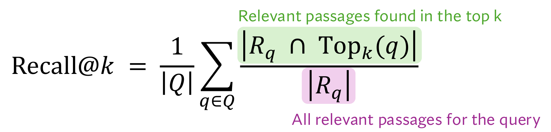
Recall@k = 1|Q|∑q ∈ Q|Rq ∩ Topk(q)||Rq|
|Rq ∩ Topk(q)|
How many right passages are in the top k. At k = 1 for q1, |{queue log}| = 1.
|Rq|
How many right passages the query has in total. For q1 that is 2, so q1's share is 1 ÷ 2 = 0.5.
Recall@k has a weakness: it never goes down as k grows, because passages only join the top k and never leave it. At k = 1,000 recall will look very high, but by lesson 2's count the holds only about 14 passages. So look at Recall@k at the k you actually put into the prompt. Recall@k also ignores the order inside the top k: whether the queue log is at rank 1 or rank 3, q1's Recall@3 is the same.
The recall of search in lesson 10 compares against the list from exact search: if 9 of the exact top 10 come back, it is 0.9. Recall@k compares against relevance labels that a person wrote.
Stanford's slide: the formulas for MRR@k and Recall@k. You can now read every line of it. Click the image to open it at full size.
5nDCG@k: is the most useful passage on top?
nDCG@k reduces each grade according to its rank, adds them up, and divides the sum by the sum for the best possible order. So it looks at two things together: how useful a passage is, and how high it sits. In the three metrics so far, a passage was simply right or wrong.
Think first
Reverse q1's order: office hours page (1), old forum post (0), queue log (3). Which of Hit@3, the reciprocal rank and Recall@3 changes for q1?
Show the answer
None of them. Hit is 1, the reciprocal rank is also 1 because the office hours page is right too, and Recall is 2 of 2. But for the reader this list is worse, because the crowd data is now at rank 3.
A first attempt could be to add up the grades in the top k. But the original order gives 3 + 0 + 1 = 4, and the reversed order gives 1 + 0 + 3 = 4, so the sum sees the grades but not the order. That is why each grade is reduced according to its rank, so that a lower passage counts for less.
Dividing by log2(rank + 1)
The reduction divides each grade by (rank + 1). log2 x answers the question: to what power must you raise 2 to get x? 21 = 2, 22 = 4 and 23 = 8, so log2 2 = 1, log2 4 = 2 and log2 8 = 3. The log2 of 3 lies between 1 and 2, because 3 lies between 2 and 4: log2 3 = 1.585. Check: 21.585 = 3.000.
This is the same idea as from lesson 4, where the base was e, about 2.718, and here it is 2. The 1 is added to the rank so that rank 1 has the divisor log2 2 = 1, and the top passage keeps its full grade:
Rank
log2(rank + 1)
Share of the grade that counts
1
log2 2 = 1
1 ÷ 1 = 1
2
log2 3 = 1.585
1 ÷ 1.585 = 0.631
3
log2 4 = 2
1 ÷ 2 = 0.5
Now work out the sum for q1's original order:
Rank 1, queue log: 3 ÷ 1 = 3.
Rank 2, old forum post: 0 ÷ 1.585 = 0.
Rank 3, office hours page: 1 ÷ 2 = 0.5.
Sum: 3 + 0 + 0.5 = 3.5.
In the reversed order the office hours page is at rank 1 and the queue log at rank 3: 1 ÷ 1 + 0 + 3 ÷ 2 = 1 + 1.5 = 2.5. Now the order shows, because 3.5 and 2.5 differ. This sum is called the , the discounted cumulative gain. Gain means the grade, cumulative means added up, and discounted means reduced by rank.
Dividing by the IDCG: bringing every query between 0 and 1
One problem remains: how large the DCG can get depends on the query. q1 has two right passages, with grades 3 and 1, so its DCG can reach 3.631. q3 has one right passage, with grade 2, so its DCG can never go above 2. A plain average would give more weight to queries with more right passages.
So each query's DCG is divided by the DCG of the best possible order for that same query, called the IDCG, the ideal DCG. q1's best order is queue log (3), office hours page (1), so IDCG = 3 ÷ 1 + 1 ÷ 1.585 = 3.631. This order comes from all the labels, not from the retriever's list, which is why q3's IDCG is 2.
Now the original order gives 3.5 ÷ 3.631 = 0.964, and the reversed order gives 2.5 ÷ 3.631 = 0.689. This ratio is called nDCG, where the n stands for normalized. It always lies between 0 and 1, and 1 means no better order is possible.
Hit, the reciprocal rank and Recall missed the reversed order, but nDCG fell from 0.964 to 0.689. The formula holds the same arithmetic, followed by the average of every query's nDCG:
Here relq,i is the grade of the passage at rank i, which is 3, 0 and 1 in q1's original order. The same arithmetic works for the other two queries. q3's right passage is not in the top 3, so its DCG is 0, and its nDCG is 0 too.
Query, k = 3
DCG
IDCG
nDCG
q1queue log (3), forum post (0), office hours page (1)
3.5
3.631
0.964
q2project page (0), syllabus (3), Homework 1 (0)
?
3
?
q3syllabus (0), Homework 1 (0), project page (0)
0
2
0
Work out the second row
q2's right passage, the syllabus (grade 3), is at rank 2. What are its DCG and nDCG? Then work out nDCG@3 over all three queries.
Show the answer
DCG = 3 ÷ log2 3 = 3 ÷ 1.585 = 1.893. IDCG = 3 ÷ 1 = 3, because the best order would put the syllabus at rank 1. nDCG = 1.893 ÷ 3 = 0.631.
nDCG@3 = (0.964 + 0.631 + 0) ÷ 3 = 0.532.
Change q1's order
Press “Up” to move a passage up one rank, and change k. The right passages have a coloured border. Build the reversed order and watch nDCG drop to 0.689.
Metric (q1 only)
Value
Stanford's slide: the formulas for Hit@k, Failed@k and nDCG@k. You can now read every line of it.
One retriever, four numbers
Now put the starting retriever's four numbers side by side. The list is the same and k = 3, yet four different numbers come out:
Query
Hit@3
Reciprocal rank
Recall@3
nDCG@3
q1
1
1
1
0.964
q2
1
0.5
1
0.631
q3
0
0
0
0
Average
0.667
0.5MRR@3
0.667
0.532
Now look at the improvement from the start once more. When q2's syllabus moves to rank 1, its nDCG becomes 3 ÷ 3 = 1, and nDCG@3 = (0.964 + 1 + 0) ÷ 3 = 0.655. MRR@3 also becomes 0.667, while Hit@3 and Recall@3 stay at 0.667.
The cost of nDCG is that it needs grades, which are even more expensive than right-or-wrong labels. The late chunking scores in lesson 8 were this nDCG@10, written as percentages. Each metric answers a different question:
Metric
The question it answers
When to use it
Hit@k, Failed@k
Did the reader get at least one right passage?
To measure the recall ceiling
MRR@k
How high is the first right passage?
When one right passage is enough
Recall@k
How many of the right passages arrived?
When the answer is spread over several passages
nDCG@k
Are the more useful passages on top?
When you have grades and the order matters
Think first
A support bot puts the top 5 passages into its prompt, and most answers sit in a single passage. Retriever A has its first right passage at rank 2 for every query. Retriever B has it at rank 1 for half the queries and outside the top 5 for the other half. Work out MRR@5 and Hit@5 for both. Which one would you choose?
Show the answer
MRR@5: A = 0.5, and B = (1 + 0) ÷ 2 = 0.5, so they are equal. Hit@5: A = 1.0, and B = 0.5.
Choose A. A brings a right passage to the reader for every query, while B gives it nothing for half of them. Looking at MRR alone, you would never see this difference.
From here: the Stanford level
The 5 steps above are the same as in the easy version. The 5 steps below take you to the level of the Stanford slides. First come every symbol on the slides and the rules of sets, then the maths of the discount and the ideal DCG. After that come averaging over queries and the nDCG@10 chart, then these metrics in the course's papers, and finally you read the slides yourself. Every piece of maths is explained where it first appears.
6The slides' symbols, and the rules of sets and 𝟙
So far each metric came on its own. Stanford's two slides write all five formulas in one shared language: sets, 𝟙, and an average over queries. The table below ties each symbol to a number from our example:
Symbol
Meaning
In our example
Q
The set of all test queries
{q1, q2, q3}
q ∈ Q
One query in Q. ∈ means “is a member of this set”.
q1
|Q|
How many queries Q holds
3
Rq
The set of right passages for query q, from the labels
1 if the condition in the brackets is true, 0 if not
𝟙[Rq3 ∩ Top3(q3) ≠ ∅] = 0 for q3
rankq
The rank of the first right passage
2 for q2
i and relq,i
A rank from 1 to k, and the grade of the passage at that rank
relq2,2 = 3 for q2
1|Q| ∑q ∈ Q
Add every query's number and divide by |Q|, which is the average
÷ 3
One thing to keep in mind: in lesson 3, |a| was the length of a vector, but here |A| is the size of a set. The bars look the same, and the meaning depends on whether a vector or a set sits inside them.
Why Failed@k = 1 − Hit@k always holds
The slide's Failed@k formula is the same as Hit@k, except that the condition says = ∅ instead of ≠ ∅. First run it directly on our numbers:
q1: Rq1 ∩ Top3(q1) = {queue log, office hours page}, which is not empty, so 𝟙[ = ∅] = 0.
q2: {syllabus}, also not empty, so 0.
q3: ∅, so 1.
Average: (0 + 0 + 1) ÷ 3 = 0.333.
That equals 1 − 0.667, and it is no coincidence. For every query exactly one of the two conditions holds, because a set is either empty or not. So for every query 𝟙[ = ∅] + 𝟙[ ≠ ∅] = 1, and over the three queries these add up to 3. Divide by 3, and Failed@k + Hit@k = 1. Check: 0.333 + 0.667 = 1.
Three facts that follow from sets
The first fact needs one more sign. means that everything in A is also in B, and A is called a subset of B. For example, Top3(q1) ⊆ Top5(q1), because the top 5 holds the three passages of the top 3 plus two more.
Recall@k never goes down, and never goes above 1. Top3 ⊆ Top5, so Rq ∩ Top3 ⊆ Rq ∩ Top5, and the bigger set cannot be smaller in size. Also Rq ∩ Topk ⊆ Rq, so the top of the fraction cannot exceed the bottom.
For a query with a single right passage, Recall@k and Hit@k are equal. If |Rq| = 1, then |Rq ∩ Topk| is either 0 or 1, and the division is by 1. q2 and q3 are such queries, and both their Recall@3 and Hit@3 are 1 and 0. This is why lesson 8's 1 minus recall@20 is Failed@20.
For each query, the reciprocal rank is never larger than Hit. 1 ÷ rankq is at most 1, and both are 0 when nothing is found. So MRR@k ≤ Hit@k.
Think first
Work out MRR@1 and Hit@1 for the list before the improvement. Why are they equal?
Show the answer
Only q1's first passage is right, so both are (1 + 0 + 0) ÷ 3 = 0.333. At k = 1, a right passage that is found must sit at rank 1, so the reciprocal rank is either 1 or 0. A difference appears only when k is larger.
There is also an edge case. If a query has no right passage in the corpus at all, then Rq = ∅ and |Rq| = 0. Recall would then divide by 0, which is impossible, and the IDCG in nDCG is 0 as well. So every query in a test set needs at least one right passage.
7The maths of the discount: logs, the harmonic series and the ideal DCG
Step 5 divided each grade by log2(rank + 1), while MRR simply takes 1 ÷ rank. Put the two discounts side by side over 10 ranks, and the difference shows:
Rank
1 ÷ rank
log2(rank + 1)
1 ÷ log2(rank + 1)
1
1
1
1
2
0.5
1.585
0.631
3
0.333
2
0.5
4
0.25
2.322
0.431
5
0.2
2.585
0.387
6
0.167
2.807
0.356
7
0.143
3
0.333
8
0.125
3.170
0.315
9
0.111
3.322
0.301
10
0.1
3.459
0.289
1 ÷ rank falls very fast: to half at rank 2, and to 0.1 at rank 10. 1 ÷ log2(rank + 1) falls slowly: it reaches half only at rank 3, and still keeps 0.289 at rank 10. So nDCG still counts the lower ranks, while a 1 ÷ rank discount almost ignores them.
The 2002 paper by Järvelin and Kekäläinen gives exactly this reason. The discount should shrink with rank, but not as steeply as dividing by the rank, so that a user who keeps reading further down still counts. Their example: log2 1024 = 10, so a document at rank 1024 still keeps a tenth of its value. Under 1 ÷ rank it would keep only 1 ÷ 1024 = 0.001. from the paper
The harmonic series, and the divisor in nDCG
The list 1, 1/2, 1/3, 1/4, … is called the , and MRR's reciprocal ranks are exactly these numbers. Their running sum grows very slowly: the first 10 add up to 2.929, the first 100 to 5.187, and the first 1,000 to 7.485. A rule shows here: the sum of the first n is about ln n + 0.577, where 0.577 is a fixed number. Check: ln 1000 = 6.908, and 6.908 + 0.577 = 7.485.
So the harmonic sum grows like a log. The same link shows up from the other side in the divisor of nDCG. Logs follow a rule you met with ln in lesson 4: log2(a × b) = log2 a + log2 b. Since 4 = 2 × 1.5 × (4 ÷ 3):
log2 2 = 1, the divisor at rank 1.
log2 1.5 = 0.585, the step from rank 1 to rank 2.
log2(4 ÷ 3) = 0.415, the step from rank 2 to rank 3.
Sum: 1 + 0.585 + 0.415 = 2 = log2 4, the divisor at rank 3.
At rank i the divisor grows by a step of log2(1 + 1 ÷ i): 1, 0.585, 0.415, 0.322, and 0.138 at rank 10. Compare these with the harmonic numbers 1, 0.5, 0.333, 0.25 and 0.1. Each step is equal to 1 ÷ i or a little bigger, and for large i it is about 1.443 ÷ i, as at i = 100, where both are 0.0144. Here 1.443 = 1 ÷ ln 2.
So the divisor in nDCG grows by shrinking steps like those of the harmonic series, while the divisor of 1 ÷ rank grows by a full 1 at every rank. That is why the log discount falls slowly.
The paper's original formula
The slide's log2(i + 1) is the later, common form. The 2002 paper divided by logb i, the log of the rank in base b. At rank 1 the log is 0, so the paper applies no discount to ranks below b. With b = 2, ranks 1 and 2 both keep their full grade, because log2 2 = 1, and rank 3 is divided by log2 3 = 1.585. from the paper
The paper's own example starts with grades 3, 2, 3, and gives a DCG of 3 + 2 + 3 ÷ 1.585 = 6.89 at rank 3, which is also the number printed in the paper. The same formula gives q1's original order (3 + 0 + 1 ÷ 1.585) ÷ (3 + 1) = 0.908, and the reversed order (1 + 0 + 3 ÷ 1.585) ÷ 4 = 0.723. my arithmetic for q1
The slide's formula gave 0.964 and 0.689 for the same two lists. The numbers changed, but both formulas rank the original order higher. So read an nDCG number only when you know which formula produced it.
The paper describes base 2 as a model of an impatient user and base 10 as a model of a persistent one. It also tried other gains in place of the grades, for example treating grades 0, 1, 2 and 3 as 0, 1, 10 and 100. from the paper With those gains, q1's original order gives 0.999 and the reversed order 0.507, because the grade-3 queue log now weighs 100 times as much as anything else. my arithmetic
The ideal DCG: built from all the labels, and cut at k
Two rules build the IDCG, and both show in our example.
The best order comes from all the labels, not from the retriever's list. The paper says the same: the ideal rests on all the relevant documents for the topic, not on the output of some system. from the paper That is why q3's IDCG is 2, even though the retriever never returned the office hours page.
IDCG@k takes only the k largest grades. Suppose a query has 4 right passages, with grades 3, 3, 2 and 1. Then IDCG@3 = 3 + 3 ÷ 1.585 + 2 ÷ 2 = 5.893, and the grade-1 passage gets no place in the top 3. IDCG@4 is 6.323. my grades
Think first
For q1 the retriever returns only the queue log at rank 1, and the other four passages are wrong. What is nDCG@3? What would happen if the IDCG were built from the retriever's list?
Show the answer
DCG = 3 ÷ 1 = 3, and the IDCG from all the labels is 3.631, so nDCG = 3 ÷ 3.631 = 0.826. If the IDCG came from the list, the best order of that list would also give only 3, and nDCG would be 3 ÷ 3 = 1. Missing the office hours page would then cost nothing.
8Averaging over queries, percentages and points, and the nDCG@10 chart
All five formulas end with 1 ÷ |Q| and ∑, an average over the queries. In this average every query has the same weight, so q1 and q3 each contribute 1 ÷ 3. That is why step 5 first divided each query by its own IDCG, and only then took the average.
Average the DCG without that division, and you get (3.5 + 1.893 + 0) ÷ 3 = 1.798. Whether that is good or bad is hard to say, because the DCG has no fixed upper limit. On top of that, q1 alone supplies 3.5 of the total 5.393, a share of 0.649. nDCG@3 = 0.532 can be read directly: on average, the lists earned 53.2% of the DCG of the best possible order.
Even so, one average can hide a lot. Retriever C gives every query an nDCG of 0.5, and retriever D gives half the queries 1 and the other half 0. Both average 0.5, but D gives the reader nothing for half the queries. my example So look at Failed@k next to the average, which was also the lesson of the support bot in step 5.
Percentages and points
Papers often multiply these numbers by 100, writing 0.532 as 53.2. In the table in lesson 8, the average for 256-token chunks is 52.2 for naive chunking and 54.0 for late chunking. Now “how much better” has two answers:
The plain difference: 54.0 − 52.2 = 1.8. This is called 1.8 .
Relative to the old number: 1.8 ÷ 52.2 = 0.0345, an improvement of about 3.45%.
The paper gives both: 1.8% absolute and 3.46% relative. from the paper The table's numbers are rounded to one decimal, so a small gap like the one between 3.45% by hand and the paper's 3.46% can appear. When someone says a new method is “3% better”, ask whether that means points or a relative change.
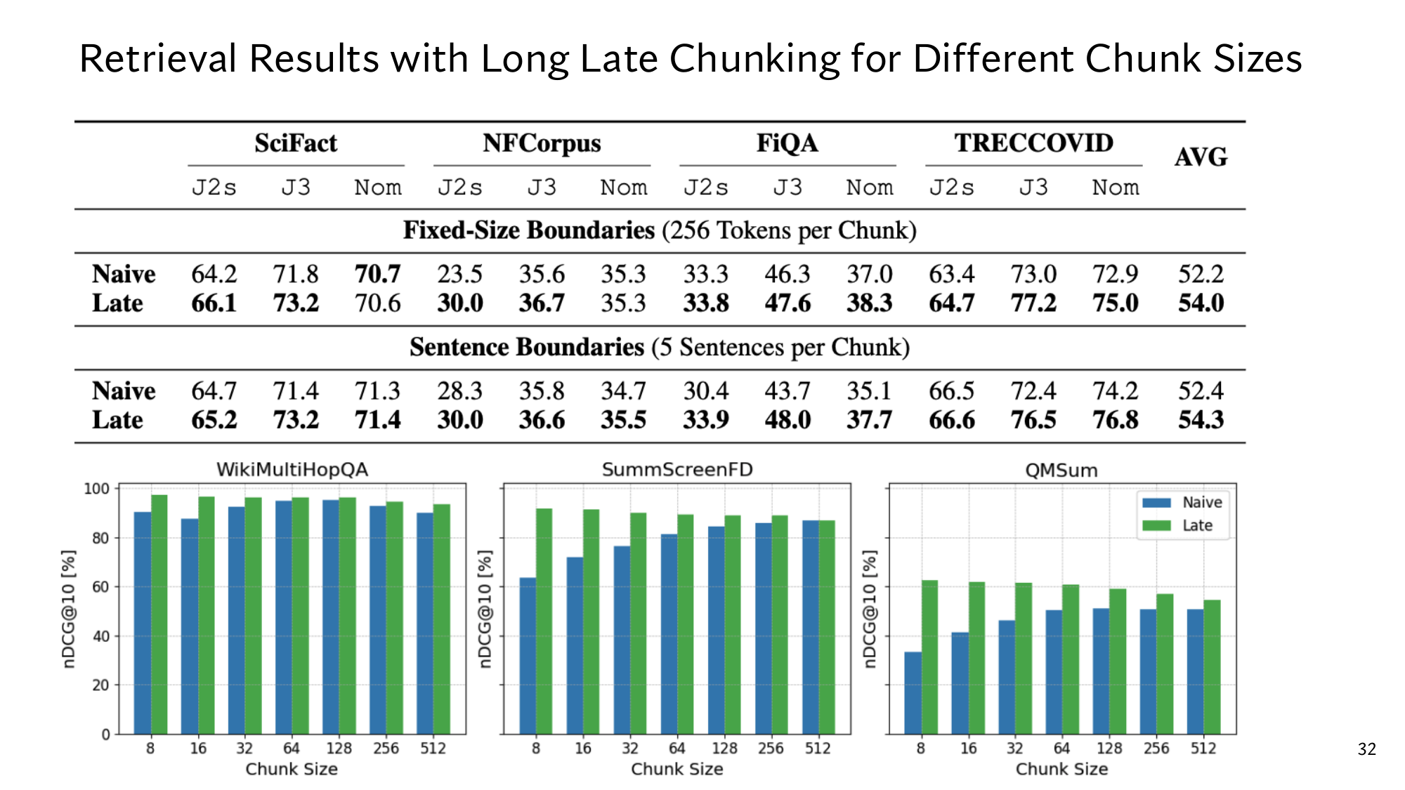
Stanford's nDCG@10 chart
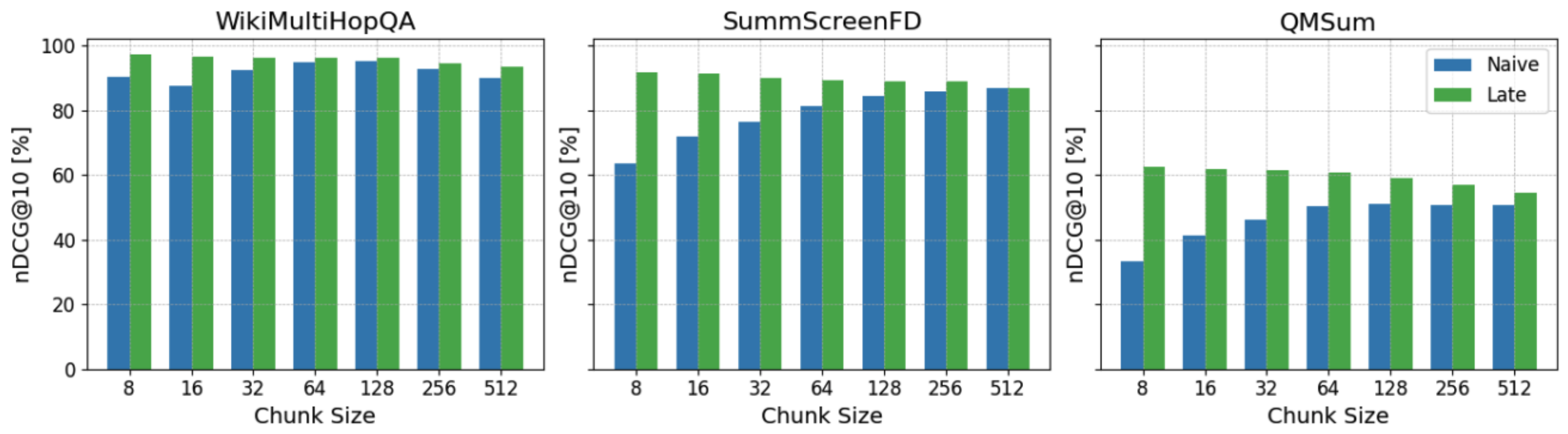
The three charts from Stanford's late chunking slide, enlarged. Blue bars are naive chunking, and green bars are late chunking.
These charts come from the late chunking paper of lesson 8. Each bar is one dataset's nDCG@10, multiplied by 100. The nDCG of the top 10 was computed for every query of that dataset, and then averaged over all its queries. So a bar at 60 means that, on average, the top-10 lists earned 60% of the DCG of the best possible order.
The paper's relevance labels are in a file, which lists the IDs of the right documents for each query. But the retriever returns chunks, not documents. So the paper replaces each chunk with its document, and when a document appears several times in the list, it keeps only its first position. from the paper That way one document cannot fill two ranks and count twice, just as a set holds each thing only once.
The x-axis is chunk size, from 8 to 512 tokens, each size double the one before. The y-axis is nDCG@10 in percent, from 0 to 100. The three datasets, WikiMultiHopQA, SummScreenFD and QMSum, come from a benchmark called LongEmbed, and the encoder is jina-embeddings-v2-small. from the paper Reading exact numbers off a chart is unreliable, so read its shape instead:
In every chart, at every chunk size, the green bar is as high as the blue one or higher. On SummScreenFD at 512 tokens the two are about equal.
The gap is largest for small chunks. On QMSum at 8 tokens the blue bar is below the 40 line, and the green bar is above 60.
On WikiMultiHopQA every bar is above 80. nDCG cannot go above 100, so there is little room left to improve.
Lesson 8 explains why late chunking wins on small chunks. For this lesson it is enough that each bar is an average over all the queries of its dataset. Every part of that average is step 5's DCG ÷ IDCG.
Think first
On some dataset, half the queries have nDCG@10 = 1 and the other half 0. Where would its bar be? Could you tell it apart, from the bar alone, from a dataset where every query has nDCG@10 = 0.5?
Show the answer
The bar would be at 50, because (1 + 0) ÷ 2 = 0.5, and 0.5 × 100 = 50. The second dataset would also be at 50, so the bar shows no difference. For that you need the numbers per query, or a number like Failed@10.
9These metrics in the course's papers
The retrieval numbers in lessons 8, 12, 14 and 15 are this lesson's metrics. The only difference is that each paper chose its labels and its k in its own way, and you need to know both before you read the number.
DPR: Hit@20 with labels made without people
The DPR paper's top-k retrieval accuracy counts the share of questions whose top-k passages contain a piece of text that answers the question. from the paper So there Rq is the set of all passages that contain the answer text, and no person picked the passages. That makes labels cheap even for 21 million passages.
The cost is that a passage counts as right even when the answer text appears in some other context. For example, q2's answer is Week 6, so any passage containing Week 6 would count as right, even one about a different deadline. my example Turn lesson 12's NQ numbers into Failed@20: 100 − 78.4 = 21.6% for DPR, and 100 − 59.1 = 40.9% for BM25. So with BM25, for 40.9% of the questions the top 20 holds no passage with the answer, and nothing useful reaches the reader.
MS MARCO: MRR@10, and reading MRR correctly
The MRR@10 numbers in lessons 14 and 15 are on the MS MARCO dataset. According to the ColBERT paper, it holds 8.8 million passages from Web pages, gathered from Bing's results for 1 million real queries. Each query has only one or very few passages marked as relevant, and no passage is explicitly marked as irrelevant. The official metric is MRR@10. from the paper
Step 6 explains this choice. When each query has a single right passage, Recall@k and Hit@k are equal, and the only question left is how high that passage sits. But “no passage marked irrelevant” also means that an unlabeled passage may well be right. A retriever that puts such a passage at rank 1 still gets 0, which is the cost of labels from step 1.
It is tempting to read MRR@10 = 0.349 as “the average rank is about 1 ÷ 0.349 = 2.9”, but that is wrong. The average of reciprocals is not the reciprocal of the average rank. Take two queries whose first right passages sit at rank 1 and rank 10: my example
1 ÷ 0.55 = 1.82, while the real average rank is (1 + 10) ÷ 2 = 5.5.
The reason is the shape of 1 ÷ x, which is the first column of step 7's table. Moving from rank 1 to rank 2 drops the reciprocal rank by 0.5. Moving from rank 9 to rank 10 drops it by only 1 ÷ 9 − 1 ÷ 10 = 0.011. So MRR mostly measures whether the first right passage is at rank 1 or 2. A passage at rank 11 counts in MRR@10 exactly like a passage that was never found: 0.
ColBERT: Recall@1000, and a recall that reranking cannot change
For retrievers that search all 8.8 million passages themselves, the ColBERT paper also reports Recall@50, Recall@200 and Recall@1000. The paper calls these numbers important for a retriever that filters a large collection down for a later step. from the paper In lesson 15, ColBERT's Recall@1000 was 96.8 and BM25's (Anserini) was 85.7, which is 11.1 points more.
One row in the same table shows the rule of sets directly. The official BM25 has a Recall@1000 of 81.4, and reranking those same top 1,000 with ColBERT still gives a Recall@1000 of 81.4. from the paper Reranking only changes the order of the same 1,000 passages, so the set Top1000 stays the same, and so does |Rq ∩ Top1000|. ColBERT searching on its own reaches a Recall@50 of 82.9, which is higher than the official BM25's Recall@1000.
The rule from step 4 applies here too: look at Recall@k at the k that the next step reads. For a reranker that reads 1,000 passages, Recall@1000 matters, and for a reader that reads about 14 passages, a number like Recall@14.
Lesson 10's recall and Recall@k
Both recalls are fractions of the same shape: |A ∩ B| ÷ |B|, the share of what should have been found that was found. The difference is in B. In the recall of lesson 10, B is the top-k vectors from exact search, and A is the ANN list. For example, if 9 of the exact top 10 come back, the recall is 9 ÷ 10 = 0.9. In Recall@k, B is Rq from the labels a person wrote.
So the ANN recall can be 1.0 while Recall@k is still 0. Suppose ANN returned exactly the vectors that exact search would. If the encoder placed the right passage's vector far away, it is not in the exact top k either. The phrase trade a little recall for a lot of speed on the lesson 10 slide is about the ANN recall.
10Now read Stanford's slides yourself
Below are this lesson's two Stanford slides, plus the late chunking slide whose charts appeared in step 8. Under each slide are a few questions. Think of the answer first, then open it. If a symbol stops you, go back to the step named in the answer. If a slide looks small on a phone, click the image to open it at full size.
Stanford's first metrics slide, and below it its two halves, enlarged.
Read the Hit@k, Failed@k and nDCG@k slide
Above Hit@k, in green, it says 1 if any relevant passage is in the top k, else 0. Which part of the formula does this, and what is its value for q3?
Show the answer
𝟙[Rq ∩ Topk(q) ≠ ∅]. q3's top 3 does not hold the office hours page, so the intersection is empty, and the value is 0. (Steps 2 and 6)
The Failed@k line ends with = 1 − Hit@k. Why does this equality hold for every retriever?
Show the answer
For each query the set is either empty or not, so 𝟙[ = ∅] + 𝟙[ ≠ ∅] = 1. Add over all queries and divide by |Q|, and Failed@k + Hit@k = 1. In our example, 0.333 + 0.667 = 1. (Step 6)
Under nDCG it says Normalized by the ideal ranking's DCG. Why is q3's IDCG 2, even though the retriever never returned the office hours page? And at rank 2, what share of the grade survives Discounted by rank position?
Show the answer
The ideal order is built from all the labels, and q3's labels contain the office hours page with grade 2, so IDCG = 2 ÷ 1 = 2. At rank 2 the divisor is log2 3 = 1.585, so a share of 0.631 of the grade counts. (Steps 5 and 7)
Stanford's second metrics slide, and below it its two formulas, enlarged.
Read the MRR@k and Recall@k slide
Counts as 0 if not in the top k: what does q3 add to MRR@3? And what does a first right passage at rank 11 add to MRR@10?
Show the answer
0 in both cases. q3 has no right passage in the top 3, and rank 11 is outside the top 10. So for MRR@10, rank 11 and “never found” are the same. (Steps 3 and 9)
The green box on Recall says Relevant passages found in the top k, and the pink box says All relevant passages for the query. What is in each box for q1 at k = 1?
Show the answer
The green box is |{queue log}| = 1, and the pink box is |{queue log, office hours page}| = 2. q1's share is 1 ÷ 2 = 0.5, and Recall@1 over the three queries is 0.5 ÷ 3 = 0.167. (Step 4)
The Average over all queries part appears in all five formulas. If a query in the test set has no right passage at all, what goes wrong in Recall?
Show the answer
Then |Rq| = 0, and you cannot divide by 0. In nDCG the IDCG is 0 as well. So every query in a test set needs at least one right passage. (Step 6)
Stanford's late chunking slide, and below it its three charts, enlarged. Lesson 8 teaches the table at the top.
Read the nDCG@10 charts
The y-axis says nDCG@10 [%]. What does a bar at 60 say in terms of nDCG?
Show the answer
For every query in that dataset the DCG ÷ IDCG of the top 10 was computed, their average is 0.6, and the chart shows it multiplied by 100 as 60. So on average the lists earned 60% of the DCG of the best possible order. (Steps 5 and 8)
The paper's labels are for documents, but the retriever returns chunks. What does the paper do before computing nDCG@10, and why?
Show the answer
It replaces each chunk with its document, and when a document appears several times, it keeps only the first position. Otherwise one right document could fill several ranks and count several times. (Step 8)
Why does the gap between green and blue look smaller on WikiMultiHopQA than in the other two charts?
Show the answer
There every bar is above 80, and nDCG cannot go above 100, so there is little room to improve. Lesson 8 explains when late chunking helps. (Step 8)
3 points from this lesson
Every metric needs relevance labels: the right passages Rq for each query, and sometimes their grades. The rules of sets and 𝟙 give Failed@k = 1 − Hit@k, and show that Recall@k never goes down as k grows.
Hit@k asks whether a right passage arrived, and MRR how high the first right passage is. Recall@k asks how many arrived, and nDCG whether the more useful passage is on top. The log discount of nDCG falls more slowly than 1 ÷ rank, so it still counts the lower ranks.
Every metric is an equal-weight average over queries, and one average can hide very different pictures. Papers take it with their own labels and k: DPR's Hit@20, MS MARCO's MRR@10 and ColBERT's Recall@1000.
New terms in this lesson
Relevance labels
The right passages fixed in advance for each query, sometimes with grades. For example, for q1 the queue log (grade 3) and the office hours page (grade 1).
Set, ∩, ∅, |A|
A group of things, the things two sets share, the empty set, and how many things a set holds. For example, |{queue log, office hours page}| = 2, and for q3, Rq3 ∩ Top3(q3) = ∅.
𝟙[condition]
1 if the condition is true, 0 if not. For example, q3's top 3 holds no right passage, so 𝟙[Rq3 ∩ Top3(q3) ≠ ∅] = 0.
Hit@k
The share of queries with at least one right passage in the top k. For example, at k = 3, 2 of 3 queries, so 0.667.
Failed@k
1 − Hit@k, the share of queries with no right passage in the top k. For example, Failed@3 = 1 − 0.667 = 0.333.
MRR@k
1 ÷ the rank of the first right passage, averaged over the queries, with 0 if none is in the top k. For example, ranks 1, 2 and none give (1 + 0.5 + 0) ÷ 3 = 0.5.
Recall@k
Right passages found in the top k ÷ all right passages, averaged over the queries. For example, at k = 1 q1 found 1 of 2, so 0.5.
log2
The power you must raise 2 to in order to get a number. For example, log2 4 = 2, and log2 3 = 1.585.
DCG and IDCG
Each rank's grade ÷ log2(rank + 1), added up. The IDCG is the DCG of the best order. For example, q1's order queue log (3), forum post (0), office hours page (1) gives DCG 3.5 and IDCG 3.631.
nDCG@k
DCG ÷ IDCG, between 0 and 1, which looks at both grade and order. For example, q1's reversed order gives 2.5 ÷ 3.631 = 0.689.
⊆ (subset)
A ⊆ B means everything in A is also in B. For example, Top3(q1) ⊆ Top5(q1), so Recall@5 is never lower than Recall@3.
Harmonic series
1 + 1/2 + 1/3 + …, the 1 ÷ rank numbers that MRR uses. Their sum grows slowly, about ln n + 0.577. For example, the first 1,000 add up to 7.485.
Points (absolute difference)
The plain difference between two percentages. For example, 52.2 to 54.0 is 1.8 points, which is an improvement of about 3.45% relative to 52.2.
QRels
A file of relevance labels: the IDs of the right documents for each query. For example, the late chunking paper computed nDCG@10 from such a file.