The job of vector search is to find the k vectors nearest to the query's vector. This lesson teaches methods that find those same k vectors most of the time without looking at every vector. The retriever in lesson 3 compared each query with every vector in the index. For the 60,000 passages of the company in lesson 2 that takes a moment, but on 100 million passages each query would take about 7.7 seconds. my estimate
The search in lesson 5 finds the k passages with the largest dot products, and the way to speed it up is the same: do not look at every vector. Then the nearest passage is sometimes missed, so this lesson also teaches you how to measure that miss.
The ladder for this lesson
The ladder has 10 steps. The first 5 are the same as in the easy version, and steps 6 to 10 take you to the level of the Stanford slides. Under each step you can see what you will be able to do after it.
What you need first: Lesson 3 (vector, dot product, length) and Lesson 9 (cluster, centroid, graph). From step 6 on, step 6 of lesson 3 (expanding the distance), Lesson 4 (ln) and Lesson 12 (DPR) also help. If you already know a step, skip to the next one. A word with a dotted underline and ▾ opens its definition when you click it.
1Comparing with every vector: exact search and its cost
Stanford's slide states the task of vector search like this: for a query vector, return the top-k of the N vectors in the index. The simplest method computes a score against every vector and returns the vectors with the k highest scores. This is called exact search, or brute force, because it looks at everything without any shortcut.
Its cost is easy to count. The of lesson 3's query [0.8, 0.2] with the office hours page [0.9, 0.1] is 0.8 × 0.9 + 0.2 × 0.1 = 0.74. That took 2 multiplications. Vectors with d numbers need d multiplications, so comparing with N vectors takes N × d multiplications.
Real vectors have a large d: a BERT-base vector has 768 numbers, so d = 768. For speed, take a rough estimate that a computer does 10 billion multiplications per second. my speed estimate
Corpus
Multiplications per query
Time per query
The company in lesson 260,000 passages
46 million60,000 × 768
0.005 second
Wikipedia in lesson 521 million passages
16.1 billion21 million × 768
1.6 seconds
A large corpus100 million passages
76.8 billion100 million × 768
7.7 seconds
The last row takes two steps:
Multiplications per query: 100 million × 768 = 76.8 billion.
Time: 76.8 billion ÷ 10 billion per second = 7.68 seconds, about 7.7 seconds.
The slide writes this cost as O(N·d), and this notation is called Big-O. Big-O does not give an exact count. It tells you how the cost grows as N or d grows. O(N·d) means that if N doubles, the cost doubles, and if d doubles, it also doubles. In the table N went from 60,000 to 100 million, about 1,667 times as many, and the time went from 0.005 to 7.7 seconds, the same factor.
Brute force always returns the true top-k, so on a small corpus it is the best method. The trouble is only on a large corpus, where each query takes seconds.
2ANN: give up a little recall for a lot of speed
Without looking at every vector you cannot be sure of the top-k, because the vector you skipped might be the nearest one. So on a large corpus you have to make a trade: look at fewer vectors, and get the right answer most of the time. The vectors nearest to a query are called its nearest neighbors.
ANN, approximate nearest neighbor search, is the family of methods that look at only a few vectors and still return the true nearest neighbors most of the time. Approximate means nearly. The slide calls it a trade: trade a little recall for a lot of speed.
Here means: of the true top-10 that brute force would return, how many did the ANN return? If the ANN returned 9 of the 10, the recall is 9 ÷ 10 = 0.9. A passage the ANN drops never reaches the reader. So this miss pushes down the from lesson 2.
Recall@k in lesson 13 is a different thing. There the right answer comes from human labels, and here it comes from brute force's top-10.
Distance: how to measure “near”
To measure “near”, the methods in this lesson use distance. To find the distance between two vectors, first subtract the numbers in the same positions, which gives a difference vector. Then take its , the calculation from lesson 3: square each number, add the squares, then take the square root.
For lesson 3's query [0.8, 0.2] and the office hours page [0.9, 0.1], this takes three steps:
Difference: [0.9 − 0.8, 0.1 − 0.2] = [0.1, −0.1].
Sum of squares: 0.1 × 0.1 + (−0.1) × (−0.1) = 0.01 + 0.01 = 0.02. The square of a negative number is positive too.
Square root: √0.02 = 0.14. Check: 0.14 × 0.14 = 0.0196, which is about 0.02.
The syllabus [0.1, 0.9] differs by [−0.7, 0.7], and its distance is √(0.49 + 0.49) = √0.98 = 0.99. The smaller the distance, the nearer the vector, so the office hours page is nearer to the query.
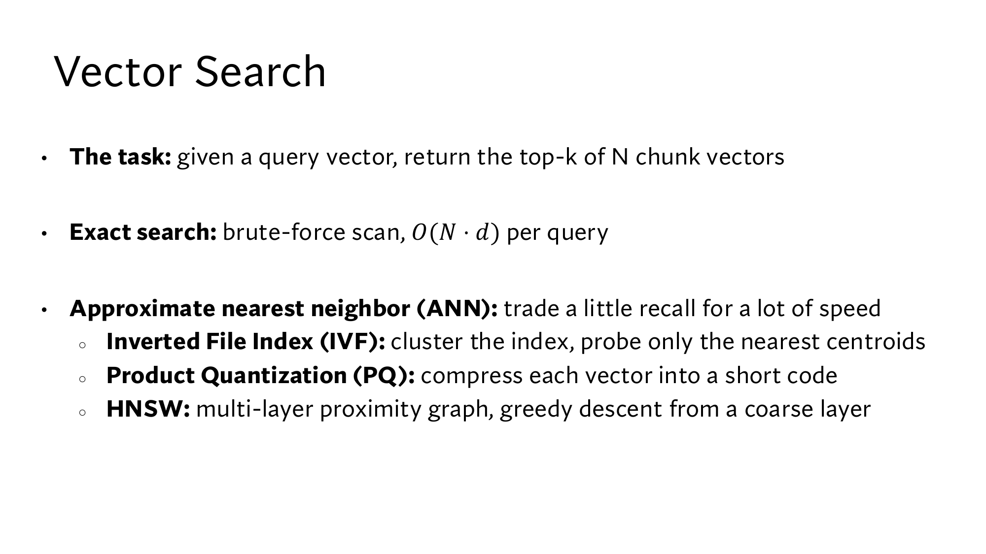
Stanford's slide: vector search. You can now read the first three lines: the task, the cost of exact search O(N·d), and the ANN trade. The three ANN methods below them, IVF, PQ and HNSW, come in the next three steps. Click the image to open it at full size.
3IVF: looking only at the clusters near the query
A query's nearest neighbors will be close to it, so looking at far-away vectors is wasted work. The difficulty is that you cannot tell a vector is far away without looking at it. Here the from lesson 9 helps, the average of a cluster's vectors. For example, the centroid of [0.1, 0.9], [0.2, 0.8] and [0.15, 0.85] is [0.15, 0.85]. If the query is far from a centroid, the vectors in its cluster are mostly far away too.
IVF (inverted file index) splits the vectors into clusters, and at search time looks only at the vectors in the clusters near the query. Its work has two parts:
: each vector goes into the cluster of its nearest centroid, and each centroid keeps a list of its vectors. These lists are called the inverted file.
Online: the query is first compared only with the centroids. IVF then picks a few of the nearest centroids and computes distances only to the vectors in their lists.
The number of clusters to look at is called nprobe. the name nprobe is not on the slide Suppose 1 million vectors are split into 1,000 clusters, about 1,000 vectors per cluster. With nprobe = 10, count the comparisons like this:
With the centroids: 1,000 comparisons.
With the vectors of the 10 chosen clusters: 10 × 1,000 = 10,000 comparisons.
11,000 in total, against 1,000,000 for brute force. 1,000,000 ÷ 11,000 = 91, so about 91 times less work.
Think first
The query sits at the edge between two clusters, and nprobe = 1. Will IVF find the true nearest point?
Show the answer
Not always. IVF looks only at the cluster whose centroid is nearest to the query. For a query at the edge, the nearest point can be in the neighbouring cluster. Pick “Query at the edge” in the widget and see.
Run IVF yourself
40 points, 4 clusters. The squares are centroids. Click the plane to place the query, and change nprobe. The dark points are the ones IVF looked at. The circled point is the true nearest one.
Pick “Query at the edge”. The centroid nearest to the query is the one on the right, so with nprobe = 1 IVF looks only at that cluster. That is 4 centroids and 11 points, 15 comparisons in total, against 40 for brute force. But the true nearest point is in the cluster on the left, and it is missed. With nprobe = 2 it is found, and the comparisons rise to 25.
This is the limit of IVF: when a query is at an edge, its nearest neighbors can be in the neighbouring cluster. “Query in the middle” even needs nprobe = 3. Raising nprobe raises recall and lowers speed, so the ANN trade is now set by a single number.
4PQ: turning each vector into a short code
IVF cut the comparisons, but all the vectors still have to sit in memory. A common number takes 4 bytes, so a vector of 768 numbers takes 768 × 4 = 3,072 bytes. 100 million vectors need 100 million × 3,072 = 307.2 billion bytes. A GB is 1 billion bytes, so that is 307 GB, about 300 GB. not on the slide
Product quantization (PQ) cuts each vector into pieces. It then replaces each piece with the number of the nearest vector in a fixed list. That list is called a codebook, and each vector in it a codeword. These numbers together make the vector's code, and the index stores this code instead of the real numbers. That is what quantization means: replacing a value with the nearest value from a fixed list.
Take the 4-number vector [0.9, 0.1, 0.2, 0.8] and cut it into two pieces: [0.9, 0.1] and [0.2, 0.8]. The codebook has 4 codewords: #0 [1, 0], #1 [0, 1], #2 [0.5, 0.5] and #3 [0.7, 0.7]. Here both pieces share one codebook, while real PQ has a separate codebook for each piece position. my example
Codeword
Distance from [0.9, 0.1]
Distance from [0.2, 0.8]
#0 [1, 0]
0.14
1.13
#1 [0, 1]
1.27
0.28
#2 [0.5, 0.5]
0.57
0.42
#3 [0.7, 0.7]
0.63
0.51
The first distance works out as [1 − 0.9, 0 − 0.1] = [0.1, −0.1], and √(0.01 + 0.01) = 0.14. The nearest codeword to the first piece is #0, and to the second piece #1. So the whole vector becomes just the code (0, 1).
From the code you can rebuild the vector roughly: #0 and #1 side by side give [1, 0, 0, 1]. Now look at the dot product with the query [1, 0, 0, 1]. With the real vector it is 1 × 0.9 + 0 × 0.1 + 0 × 0.2 + 1 × 0.8 = 1.7, and with the rebuilt vector it is 1 + 1 = 2.0.
At real scale, cut the 768 numbers into 96 pieces of 8, and give each codebook 256 codewords. A byte has 8 bits, and 8 bits make 2 × 2 × 2 × 2 × 2 × 2 × 2 × 2 = 256 different numbers. So every code from 0 to 255 fits in 1 byte, and the whole vector takes 96 bytes. common settings, not on the slide
The vector became 3,072 ÷ 96 = 32 times smaller, and 100 million vectors shrank from 300 GB to about 9.6 GB. The arithmetic: 100 million × 96 = 9.6 billion bytes, which is 9.6 GB.
The limit shows in the 1.7 and 2.0 above: a score from a code is an estimate, and close scores can swap order. That is why many systems score the last few candidates again with their real vectors.
Think first
With the codebook above, what is the code of the vector [0.65, 0.65, 0.95, 0.05]?
Show the answer
The nearest codeword to [0.65, 0.65] is #3 [0.7, 0.7], at distance 0.07. #2 [0.5, 0.5] is 0.21 away. The nearest to [0.95, 0.05] is #0 [1, 0], at distance 0.07. Code = (3, 0).
5HNSW: a greedy walk on a layered graph
IVF misses at the edges because it never looks at the vectors in the other clusters. A second idea builds no clusters at all: it connects each vector to a few of its nearby vectors. Such a graph is called a proximity graph, and every vector in it is a node, as in the graph from lesson 9.
A search on a proximity graph starts at one node, and at every step moves to the neighbor nearest to the query. When no neighbor is nearer than the current node, the search is stuck, and that node is the answer. This walk is called greedy search.
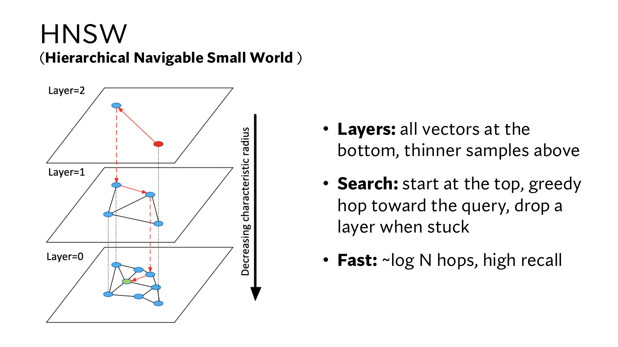
On a single layer, starting far away means many small steps. So HNSW (Hierarchical Navigable Small World) builds the graph in layers. Layer 0 holds every vector, and the layers above hold fewer nodes with longer jumps between them. The search starts at the top, and wherever it gets stuck, it drops down one layer.
So that you can do the arithmetic by hand, take a 1-dimensional example. The vectors are 21 numbers from 0 to 100, spaced 5 apart, and the distance is just the difference between two numbers. Each node is linked to its left and right neighbors in its layer. The query is 73, and the search starts at node 10 in layer 2. my example
Layer 2: 10, 50, 90
Layer 1: 10, 30, 50, 70, 90
Layer 0: 0, 5, 10, …, 100 (all 21)
Layer
At (distance)
Neighbors (distance)
Decision
2
10 (63)
50 (23)
Move to 50
2
50 (23)
10 (63), 90 (17)
Move to 90
2
90 (17)
50 (23)
Stuck, drop to layer 1
1
90 (17)
70 (3)
Move to 70
1
70 (3)
50 (23), 90 (17)
Stuck, drop to layer 0
0
70 (3)
?
?
0
75 (2)
70 (3), 80 (7)
Stuck. Answer: 75
Work out the sixth row
On layer 0 you are at node 70. Who are its neighbors, how far are they from the query 73, and what is the decision?
Show the answer
Layer 0 holds all 21 numbers, so 70's neighbors are 65 and 75. Distances: 65 (8) and 75 (2). 75 is nearer than the current node 70 (3), so move to 75.
It took 4 steps in total (50, 90, 70, 75), and the answer is right, because 75 is the nearest number to 73. Along the way the search computed the distance to 7 nodes, while brute force would compute all 21.
As N grows, this gap grows a lot. The slide says HNSW takes about steps, roughly the number of times you multiply 2 by itself to reach N. Multiplying 2 by itself 20 times gives 1,048,576. So 1 million vectors take about 20 steps, and 100 million about 27.
Stanford's slide: the layers of HNSW. The red point is the starting node at the top, the red arrows are the greedy walk, and the red dashed arrows show where the search dropped down a layer. The green point is the query. The arrow on the right says that edges get shorter in the lower layers, as in our example with jumps of 40, 20 and 5. Click the image to open it at full size.
The price of HNSW is memory, because every node also has to store its edges. not on the slide Its limit is that the greedy walk can get stuck at a node that is not the true nearest one. This happens especially when the vectors fall into separate groups. That is why HNSW also gives each new vector one edge to a different group.
From here: the Stanford level
The 5 steps above are the same as in the easy version. The 5 steps below take you to the level of the Stanford slides: first the maths of distance and dot product, then k-means for IVF's centroids, then PQ codebooks. After that come HNSW's layers, ef and the rule for choosing neighbors, and finally you read the slides yourself. Every piece of maths is explained where it first appears.
6Distance and dot product: when the two give the same order
Step 2 showed how to compute a distance. In this step you will see why that calculation is Pythagoras, and how distance is tied to the dot product. The tie matters because IVF and HNSW work with distances, while the MIPS of lesson 5 asks for the largest dot product.
Distance by Pythagoras, from 2 numbers to 768
On the plane, the query [0.8, 0.2] is one point and the office hours page [0.9, 0.1] is another. To get from the first point to the second, move 0.1 along the x-axis, then 0.1 down along the y-axis. These two moves are at 90° to each other, so they are the two short sides of a right triangle. The straight line joining the two points is the long side, and Pythagoras gives its length as √(0.1² + 0.1²) = √0.02 = 0.141.
With a third number there is one more direction, at 90° to the first two, and Pythagoras is applied twice. The result is that the square of every number in the difference is added. For example, the distance between [0.8, 0.2, 0.5] and [0.9, 0.1, 0.3] is √(0.01 + 0.01 + 0.04) = √0.06 = 0.245. my numbers The same rule holds for 768 numbers: 768 subtractions, 768 squares and 767 additions. That costs about as much as a dot product, so brute force with distances is also O(N·d).
Order without the square root
To rank passages you do not need the square root. For the office hours page the sum of squares is 0.02, and for the syllabus 0.98. Taking square roots gives 0.14 and 0.99, and the order stays the same. This always happens, because √ is an : a bigger number has a bigger square root. For the same reason the PQ paper skips square roots during search. from the PQ paper From here on, the steps also work with distance², the sum of squares.
Distance and dot product for vectors of length 1
The dense version of lesson 3 expanded distance² into a formula. There the school rule (x − y)² = x² + y² − 2xy was applied to every number, and adding everything up gave:
|a − b|2 = |a|2 + |b|2 − 2 a · b
Check it on the office hours page: |a|² = 0.8² + 0.2² = 0.68, |b|² = 0.9² + 0.1² = 0.82, and a · b = 0.74. So 0.68 + 0.82 − 2 × 0.74 = 0.02, which is the sum of squares from above.
Now both vectors, dividing each number by the vector's length so that the length becomes 1. Then |a|² = |b|² = 1, and the formula becomes:
|a − b|2 = 2 − 2 a · b
The 2 is the same for every passage, so the larger the dot product, the smaller the distance². After normalizing, the query is [0.970, 0.243], the office hours page [0.994, 0.110] and the syllabus [0.110, 0.994]: my arithmetic
Passage
Dot product
2 − 2 × dot product
Distance² computed directly
Office hours page
0.991
0.018
0.018
Syllabus
0.348
1.304
1.304
So for vectors of length 1, the nearest vectors are exactly the ones with the largest dot product. That is why an IVF or HNSW index built on distances also does the job of MIPS for such vectors.
When the length is not 1: turning MIPS into a distance search with one extra number
In lesson 3 the FAQ page [1.6, 1.4] was first by dot product (1.56) but last by distance (1.44). So when lengths are not 1, the nearest vector and the vector with the largest dot product can differ. The FAISS paper gives a way around this: add one more number to every passage vector, and a 0 to the query. from the FAISS paper
The added number is √(α² − |y|²). Here |y|² is the passage's length squared, and α² is the |y|² of the longest passage. Among our four passages the longest is the FAQ page, with |y|² = 1.6² + 1.4² = 4.52. So take α² = 4.52.
Office hours page: |y|² = 0.82, so the added number is √(4.52 − 0.82) = √3.70 = 1.924. The new vector is [0.9, 0.1, 1.924], and the query is [0.8, 0.2, 0].
FAQ page: the added number is √(4.52 − 4.52) = 0, and distance² = 0.8² + 1.2² + 0 = 0.64 + 1.44 = 2.08.
Now the FAQ page (2.08) is nearer than the office hours page (3.72), exactly as in the dot product order. The reason is that every new passage vector has |y|² equal to α², because |y|² + (α² − |y|²) = α². The formula above then gives the new distance² = |x|² + α² − 2 x · y. |x|² and α² are the same for every passage, so the order depends only on the dot product. Check: 0.68 + 4.52 − 2 × 1.56 = 2.08.
Passage
Dot product
Old distance
New distance²
FAQ page
1.56
1.44
2.08
Office hours page
0.74
0.14
3.72
Project page
0.32
0.85
4.56
Syllabus
0.26
0.99
4.68
7k-means: where IVF's centroids come from
In step 3 IVF's centroids were already there. The most common way to make them is k-means, and the PQ paper builds its codebooks the same way. from the PQ paper In k-means, k is fixed in advance: how many clusters you want.
k-means splits the vectors into k clusters by repeating two steps. The first step gives each vector to its nearest centroid, and the second makes each centroid the average of its vectors. The whole method has four steps:
Start: pick k vectors at random and treat them as centroids.
Assign: put each vector into the cluster of its nearest centroid.
Average: make each centroid the average of the vectors in its cluster.
Repeat steps 2 and 3 until no vector changes its cluster.
Run it on 6 of the course's passages. Each vector has two numbers: how much the passage is about office hours, and how much about deadlines, as in lesson 3. Here k = 2, and the queue log and the forum post start as the centroids. Both are office hours passages, so this is a deliberately bad start. my vectors and start
Passage and vector
Round 1
Round 2
Office hours page[0.9, 0.1]
A
A
Queue log[0.85, 0.2]
A
A
Forum post[0.7, 0.3]
B
A
Syllabus[0.1, 0.9]
B
B
Project page[0.2, 0.8]
B
B
Homework 1 announcement[0.3, 0.7]
B
B
Round 1. The centroids are A = queue log [0.85, 0.2] and B = forum post [0.7, 0.3]. The syllabus [0.1, 0.9] has distance² 0.75² + 0.7² = 1.0525 to A, and 0.6² + 0.6² = 0.72 to B. So the syllabus goes to B, and so do the project page and Homework. The office hours page goes to A.
First average. A = [(0.9 + 0.85) ÷ 2, (0.1 + 0.2) ÷ 2] = [0.875, 0.15]. B, the average of four vectors, is [(0.7 + 0.1 + 0.2 + 0.3) ÷ 4, (0.3 + 0.9 + 0.8 + 0.7) ÷ 4] = [0.325, 0.675].
Round 2. The forum post [0.7, 0.3] has distance² 0.175² + 0.15² = 0.053 to A, and 0.375² + 0.375² = 0.281 to B. So the forum post moves to A, and the other five stay where they are.
Second average. A = [0.817, 0.2] and B = [0.2, 0.8].
Round 3. No vector changes cluster, so k-means stops.
In round 1, B was very large because both starting centroids sat on the office hours side. The first average moved B's centroid towards deadlines, and the forum post returned to the office hours group.
Each step of k-means lowers one number, or at least never raises it: the sum of distance² from every vector to its centroid. In our example it starts at 1.553. After the first average it is 0.421, after round 2 it is 0.193, and after the second average 0.082. Averaging lowers it because the average is the point with the smallest sum of distance² to its vectors. For example, from 0.9 and 0.85 to 0.875 this sum is 0.025² + 0.025² = 0.00125, while to 0.85 it is 0.05² + 0 = 0.0025.
Neither assigning nor averaging ever raises this sum, so k-means always stops somewhere. But where it stops is not always the best place, as the PQ paper also notes.
The PQ paper calls the two conditions behind these steps Lloyd's conditions. First, each vector goes to its nearest centroid, and second, each centroid is the average of its vectors. from the PQ paper The squares in step 3's widget meet these conditions too. Each square is exactly the average of the 10, 11, 10 or 9 points in its cluster. my arithmetic
IVF search on the k-means clusters
Now run IVF for the query [0.8, 0.2] with nprobe = 1:
Distance² to the centroids: 0.0003 to A [0.817, 0.2], and 0.72 to B [0.2, 0.8]. So IVF looks only at A.
Distance² to A's three passages: office hours page 0.02, queue log 0.0025, and forum post 0.02.
The nearest is the queue log, which is also the nearest of all 6 passages. That took 2 + 3 = 5 comparisons, against 6 for brute force.
On 6 passages the saving is small, but on the 1 million vectors of step 3 the same method did 91 times less work.
How many clusters to make
The FAISS paper gives a formula for IVF's comparisons. Suppose there are K clusters, N vectors spread evenly across them, and nprobe clusters to look at: from the FAISS paper
comparisons = K + nprobe × N ÷ K
The first part is the comparisons with the centroids, and the second is the comparisons with the vectors in the chosen clusters. Raising K raises the first part, but each cluster gets smaller, so the second part falls. Look at the table for N = 1 million and nprobe = 10:
K, the clusters
10 × N ÷ K
Total comparisons
100
100,000
100,100
1,000
10,000
11,000
3,162
3,162
6,325
10,000
1,000
11,000
100,000
100
100,100
The total is smallest where the two parts are equal: K = nprobe × N ÷ K, so K² = nprobe × N. Here K² = 10 × 1,000,000 = 10 million, and K = √(10 million) = 3,162. The 1,000 clusters of step 3 gave 11,000 comparisons, and 3,162 clusters give only 6,325.
The FAISS paper also says this is only a rough guide on real data. Clusters are not even, and with more clusters you also need a larger nprobe to keep the same recall. In the paper's experiments the fastest K came out at roughly 15 to 20 times √N. from the FAISS paper
The dense version of lesson 4 said that when the passages double, MIPS takes less than twice as long. The FAISS paper measured IVF's search time as growing like Nα, with α = 0.34 at recall 0.9. from the FAISS paper When N doubles, the time grows by a factor of 20.34. To see what that means, look at 20.5 first: 20.5 × 20.5 = 21 = 2, so 20.5 = √2 = 1.41. 0.34 is smaller than that, and 20.34 = 1.27, so the time rises by only 27%. At higher recall α rises: 0.29 at recall 0.5, and 0.45 at 0.99.
IVF takes its name from the of lesson 11. There each word keeps a list of the passages that contain it. In IVF each centroid keeps a list of the vectors in its cluster. The PQ paper sends the query to its w nearest centroids and calls this multiple assignment. That w is today's nprobe. from the PQ paper
8PQ codebooks, and fast scores from a code
A codebook comes from k-means
The codebook in step 4 was given. Real PQ builds each codebook by running k-means separately for each piece position. from the PQ paper That is, take many training vectors, run k-means with 256 centroids on their first pieces, and those centroids are the first codebook. The second pieces give the second codebook, and so on, 96 codebooks in all.
Look at it on a small scale. Take 8 training pieces that sit close together in pairs. The first pair is [0.95, 0] and [1.05, 0], and the second [0, 0.95] and [0, 1.05]. The third pair is [0.45, 0.55] and [0.55, 0.45], and the fourth [0.75, 0.65] and [0.65, 0.75].
If the start takes one piece from each pair, k-means with k = 4 makes each pair a cluster in one round. Each centroid is the average of its pair, for example [(0.75 + 0.65) ÷ 2, (0.65 + 0.75) ÷ 2] = [0.7, 0.7]. The four centroids are [1, 0], [0, 1], [0.5, 0.5] and [0.7, 0.7], exactly the codebook of step 4. my numbers
The codebooks themselves are tiny. 96 codebooks × 256 codewords × 8 numbers = 196,608 numbers, at 4 bytes each. That is 786,432 bytes, about 0.79 MB, while the codes for 100 million vectors take 9.6 GB.
Why the name says product
In the toy, each piece can take one of 4 codewords, so a code can stand for 4 × 4 = 16 different vectors. In maths, the set of all pairs from two lists is called their Cartesian product, and that is where PQ gets its name. from the PQ paper At real scale the count is 25696. 256 = 28, and a power of a power multiplies the exponents, for example (22)3 = 43 = 64 = 26. So 25696 = 28 × 96 = 2768, a number with 232 digits.
Nobody could store a list of that many vectors. PQ keeps only 96 × 256 = 24,576 codewords and can write any of those vectors by combining them.
Lookup table: a score from a code without rebuilding the vector
In step 4, to get a score from a code, we first rebuilt the vector [1, 0, 0, 1]. The PQ paper gives a faster way. The query is not turned into a code. Instead, the system computes the score of every query piece with every codeword in advance and keeps them in a table. from the PQ paper
The paper calls this asymmetric distance computation, or ADC, because the query stays exact while the passage is a code. Our query [1, 0, 0, 1] has two pieces, [1, 0] and [0, 1], and the table is:
Codeword
First piece [1, 0]
Second piece [0, 1]
#0 [1, 0]
1
0
#1 [0, 1]
0
1
#2 [0.5, 0.5]
0.5
0.5
#3 [0.7, 0.7]
0.7
0.7
Now each passage's score is just the sum of two numbers:
Code (0, 1): #0 in the first column gives 1, and #1 in the second column gives 1. The score is 1 + 1 = 2.0, the same as in step 4.
Code (3, 0): 0.7 + 0 = 0.7. Its real vector [0.65, 0.65, 0.95, 0.05] has a dot product of 0.65 + 0.05 = 0.70.
The table works because the dot product of a whole vector is the sum of the dot products of its pieces. Distance² is also the sum of the pieces' distance², and the PQ paper builds the same table with distance². At real scale the arithmetic is:
Table: 96 pieces × 256 codewords = 24,576 numbers. Building it takes 256 × 768 = 196,608 multiplications, once per query.
Each passage: pick 96 numbers from the table and add them up. With the real vector it took 768 multiplications.
100 million passages: 100 million × 96 = 9.6 billion additions, against 76.8 billion multiplications with the real vectors. On top of that, 32 times less data has to be read from memory.
The PQ paper says that each distance needs only m additions, where m is the number of pieces. The paper also has a method that turns the query into a code too, SDC. But it prefers ADC, because its distances are more precise. from the PQ paper
IVF and PQ together: the code of a residual
The PQ paper combines IVF and PQ and calls the combination IVFADC. from the PQ paper Here a vector's code is not made directly. First subtract the centroid of the vector's cluster, then make the code of the difference that is left. That difference is called the residual.
The centroid of cluster A in step 7 is [0.817, 0.2]. The residual of the queue log [0.85, 0.2] is [0.033, 0], of the office hours page [0.9, 0.1] it is [0.083, −0.1], and of the forum post [0.7, 0.3] it is [−0.117, 0.1]. These numbers are much smaller than the real vectors, so 256 codewords can cover a small region densely. The paper also says that the code of a residual is more precise than the code of the vector itself.
The paper mostly uses m = 8 pieces and 256 codewords, so each code is 8 bytes, or 64 bits. Its SIFT image vectors have 128 numbers, which is 128 × 4 = 512 bytes, so the code is 64 times smaller. For IVF the paper uses 1,000 to 1 million clusters, and it also tests the method on 2 billion vectors. The paper re-ranks the last R candidates with the exact distance, and tries R = 10, 100 and 1,000. from the PQ paper
9HNSW: random layers, ef and the rule for choosing neighbors
How high each node goes
The HNSW paper picks each new node's top layer at random, with a chance of 1/M of reaching each next layer. from the HNSW paper Take M = 16. Then each node reaches layer 1 with chance 1/16, 1/16 of those reach layer 2, and so on. For 100 million nodes the counts work out like this: my arithmetic
Reaches at least layer
Arithmetic
Nodes
0
all
100,000,000
1
100 million ÷ 16
6,250,000
2
÷ 256
390,625
3
÷ 4,096
24,414
4
÷ 65,536
1,526
5
÷ 1,048,576
95
6
÷ 16,777,216
6
On average 0.37 nodes reach layer 7, so usually none do. The top layer is therefore about 6. This count is log16 N, the number of times you multiply 16 by itself to reach 100 million: 6.64 times.
Step 5 used log2, which is 26.6 for 100 million. 16 = 24, so each multiplication by 16 equals 4 multiplications by 2, and log16 N = log2 N ÷ 4 = 26.6 ÷ 4 = 6.64. The slide's ~log N gives no base, because changing the base only changes a fixed factor. It was the same with ln and log10 in lesson 4.
The HNSW paper's argument has two parts. from the HNSW paper The average number of steps on each layer stays below a fixed number, however large N is. And the number of layers grows like log N, as the table above shows. So the total number of steps also grows like log N. The paper shows this firmly for low-dimensional data, and leaves it as an open question for high dimensions such as 128.
The paper's formula: l = ⌊−ln(U) × mL⌋
The paper picks each new node's layer l with this formula: from the HNSW paper
l = ⌊ −ln(U) × mL ⌋, where mL = 1 ÷ ln M
U is a random number between 0 and 1. For M = 16, 16 = 2.773, so mL = 0.361. ⌊x⌋ means dropping the decimal part of x, for example ⌊2.10⌋ = 2. Here are three random draws:
U = 0.5: −ln 0.5 = 0.693, and 0.693 × 0.361 = 0.25. ⌊0.25⌋ = 0, so the node stays only in layer 0.
U = 0.05: −ln 0.05 = 2.996, and 2.996 × 0.361 = 1.08. The node goes up to layer 1.
U = 0.003: −ln 0.003 = 5.809, and 5.809 × 0.361 = 2.10. The node goes up to layer 2.
A node reaches layer 1 when −ln(U) × mL is at least 1. Multiply both sides by ln 16, and the condition becomes −ln U ≥ ln 16. By lesson 4's rule ln(a ÷ b) = ln a − ln b, −ln U = ln(1 ÷ U). ln is an increasing function, so the condition means 1 ÷ U ≥ 16, that is, U ≤ 1/16 = 0.0625.
The chance that U is below 0.0625 is exactly 1/16. In the same way, layer 2 needs U ≤ 1/256 = 0.0039. The draw 0.05 meets the first condition, and 0.003 meets both. The paper calls mL = 1/ln M a simple and good choice.
ef: several candidates instead of one
The greedy walk of step 5 remembered only one node at a time. On layer 0, the HNSW paper's search keeps a list of the ef nearest nodes found so far. It looks at the neighbors of all of them. from the HNSW paper On the upper layers ef = 1, so the walk there is the same greedy walk. A larger ef means more distances computed, but higher recall. So in HNSW, ef does the job that nprobe does in IVF.
In step 5's example, start at node 70 on layer 0 with ef = 3. The list holds at most 3 nodes. Each time, the search takes the nearest node in the list whose neighbors it has not yet looked at: my example
70 (3) has neighbors 65 (8) and 75 (2). The list is not full yet, so both come in: {75, 70, 65}.
75 has neighbors 70 and 80. 70 is already in the list, and 80 (7) is nearer than the list's farthest node 65 (8). So 80 comes in and 65 drops out: {75, 70, 80}.
80's new neighbor 85 (12) is farther than the list's farthest node 80 (7), so it does not come in.
The remaining candidate 65 (8) is also farther than the list's farthest node 80 (7), so the search stops.
The result is {75, 70, 80}, which is exactly the true top-3 for the query 73: 75 (2), 70 (3) and 80 (7). With ef = 1 the search would return only 75. The paper's search algorithm returns the k nearest nodes from the list at the end, so ef must be at least k. DPR set the search depth of its FAISS HNSW index to 128, and that is ef. from the DPR paper
The rule for choosing neighbors, so the walk does not get trapped
In the easy version each new node linked to its M nearest nodes. The HNSW paper uses a better rule, which it calls a heuristic. from the HNSW paperLook at the candidates from nearest to farthest. Link a candidate only if it is nearer to the new node than to every node already linked.
Take an example. The new node is X = [3, 0], and M = 2. Cluster 1 has A [2, 0], B [1.6, 0.6] and C [1.5, −0.5], and cluster 2 has E2 [6, 0]. my numbers
Candidate
Distance to X
Distance to A, already linked
Decision
A
1.00
–
Link
B
1.52
0.72
Skip
C
1.58
0.71
Skip
E2
3.00
4.00
Link
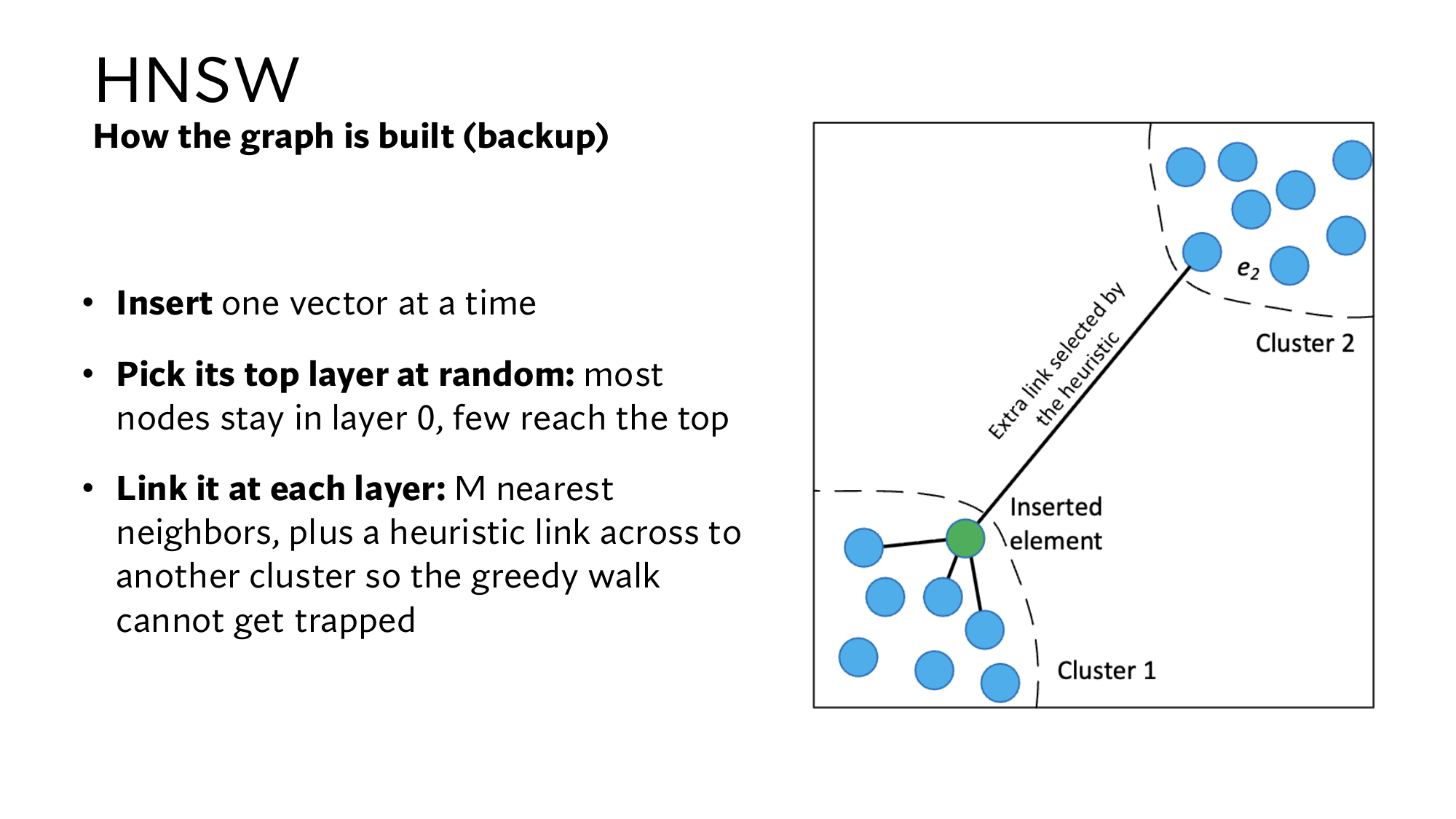
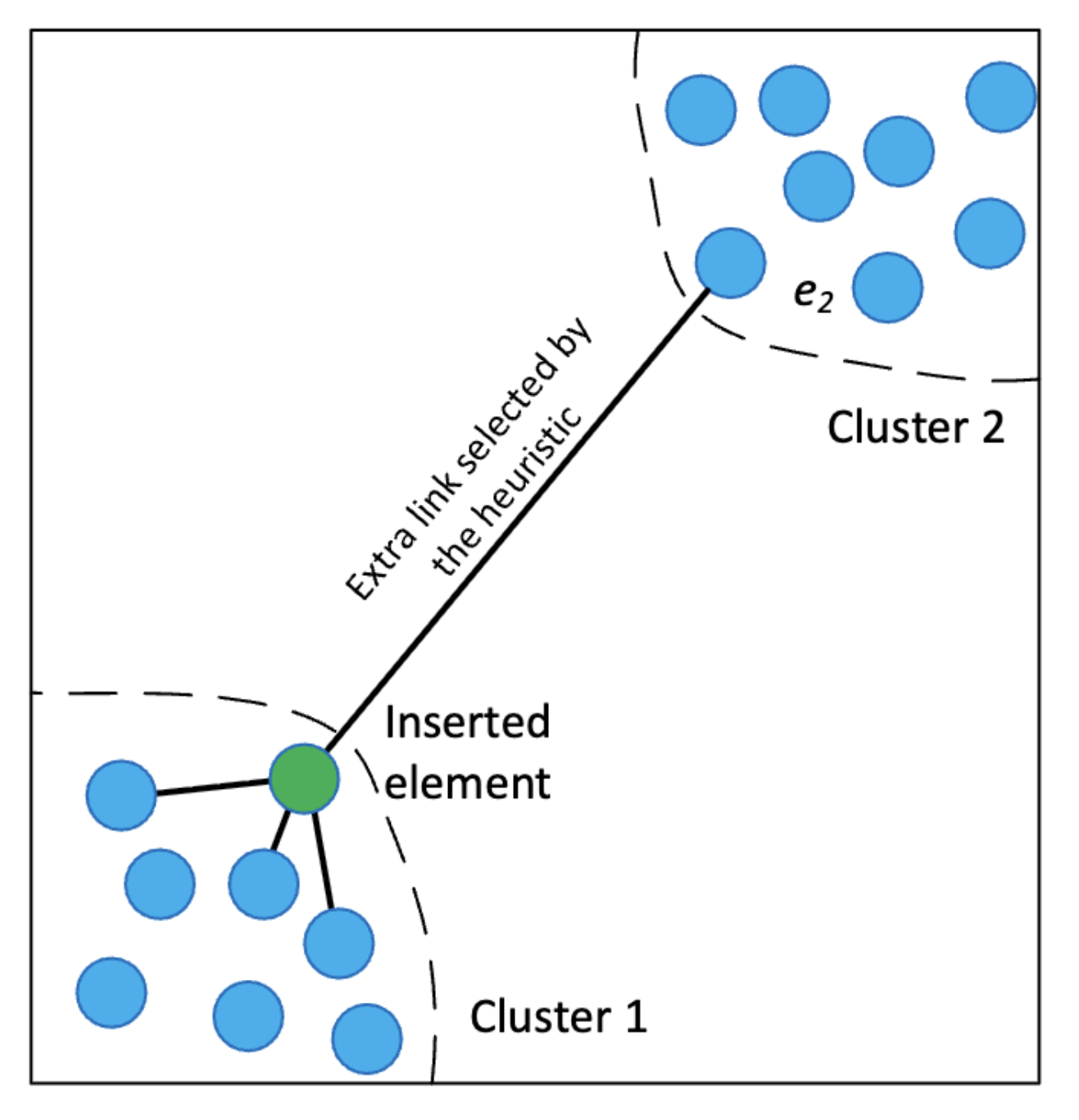
Choosing only the nearest would link X to A and B, both in cluster 1. The rule skips B and C, because both are nearer to A than to X, so they are within reach through A. E2 is far away, but even farther from A, so it lies in a new direction and gets linked. This is the “extra link” to e2 on Stanford's backup slide.
Now put two more nodes in cluster 2, F [7, 1] and G [6.4, 0.6], linked to E2 and to each other. A, B and C in cluster 1 are also linked to each other. The query is [6.5, 0.5], and the search starts at B:
At (distance)
Neighbors (distance)
Decision
B (4.90)
A (4.53), C (5.10)
Move to A
A (4.53)
B (4.90), C (5.10), X (3.54)
Move to X
X (3.54)
A (4.53), E2 (0.71)
Move to E2
E2 (0.71)
X (3.54), F (0.71), G (0.14)
Move to G
G (0.14)
E2 (0.71), F (0.71)
Stuck. Answer: G
Without the rule, X's neighbors would be A and B. The search would then go from B straight to X and get stuck there, because A and B are both farther from the query than X. The answer would be X, at distance 3.54, while the true nearest node G is at 0.14. The HNSW paper also says that with only the nearest neighbors, a search on clustered data gets stuck at cluster boundaries. Then high recall is out of reach. from the HNSW paper
Memory and scale
Most of HNSW's memory goes to edges. from the HNSW paper On layer 0 each node has at most Mmax0 edges, and the paper suggests Mmax0 = 2M. Each upper layer has Mmax edges per node, and a node sits in mL upper layers on average. Each edge is a 4-byte number, so the paper's formula is:
memory per vector = (Mmax0 + mL × Mmax) × 4 bytes
Take M = 16 and Mmax = M: Mmax = M is my assumption
Mmax0 = 2 × 16 = 32, and mL × Mmax = 0.361 × 16 = 5.77.
(32 + 5.77) × 4 = 151 bytes per vector.
For 100 million vectors that is 15.1 GB, on top of the 300 GB for the vectors themselves.
The paper considers M between 5 and 48 reasonable, and puts the memory for edges at 60 to 450 bytes per vector. Check: for M = 6, (12 + 0.558 × 6) × 4 = 61 bytes, and for M = 48, (96 + 0.258 × 48) × 4 = 434 bytes. According to the paper, a small M is better for low recall and low dimensions, and a large M for high recall and high dimensions.
Building the graph uses ef too, under the name efConstruction. When HNSW adds a new node, it finds the node's candidates with a list of this size. In the paper, an index of 10 million SIFT vectors with efConstruction = 100 took about 3 minutes on a 40-core server. For the 21 million vectors of lesson 12, DPR used 512 neighbors per node and efConstruction 200. Its index took 8.5 hours to build. from the DPR paper
10Now read Stanford's slides yourself
Below are Stanford's three vector search slides, unchanged. Under each slide are a few questions. Think of the answer first, then open it. If something stops you, go back to the step named in the answer. If a slide looks small on a phone, click the image to open it at full size.
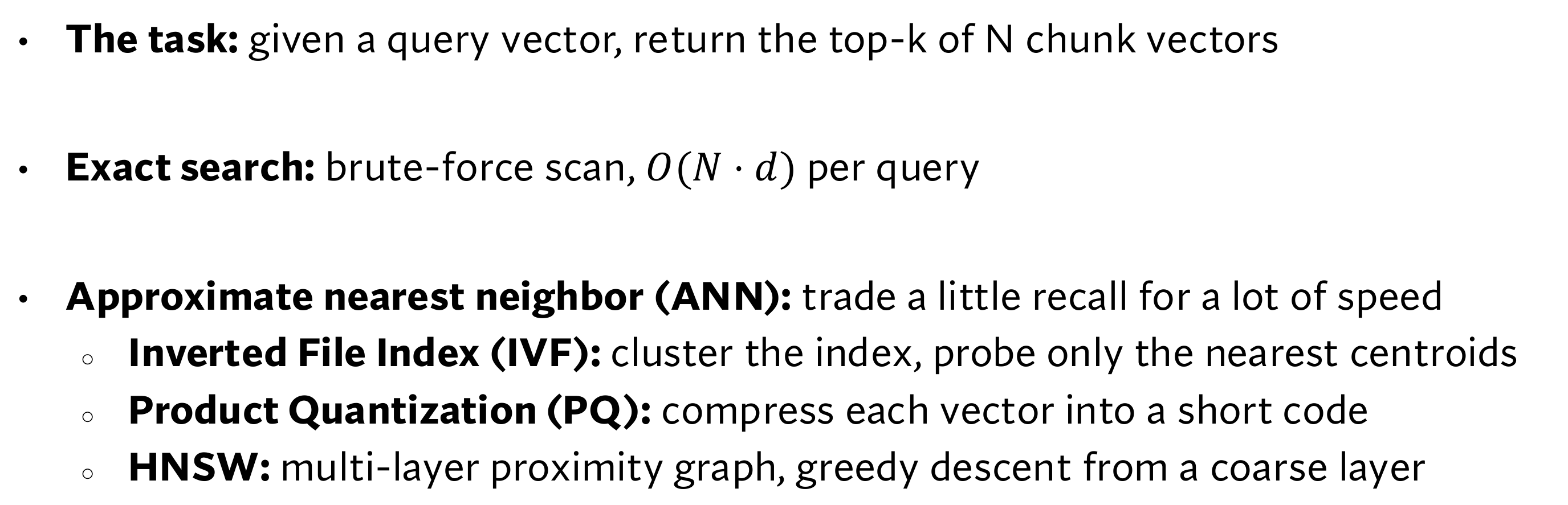
Stanford's vector search slide, and below it the text, enlarged.
Read the vector search slide
In O(N·d) per query, what are N and d? What does it mean for 100 million passages and d = 768?
Show the answer
N is the number of vectors in the index, and d is the number of numbers in each vector. 100 million × 768 = 76.8 billion multiplications, which at 10 billion per second is about 7.7 seconds per query. Distances cost the same. (Steps 1 and 6)
In “trade a little recall for a lot of speed”, recall of what? How does it differ from Recall@k in lesson 13?
Show the answer
Here recall says how many of brute force's true top-k the ANN returned, for example 0.9 for 9 out of 10. Recall@k in lesson 13 uses human labels to measure whether the correct passages made it into the top k. (Step 2)
Of IVF, PQ and HNSW, which cut the number of comparisons, and which cuts memory? Where do the centroids in the IVF line come from?
Show the answer
IVF and HNSW look at fewer vectors, so they cut comparisons. PQ cuts memory, from 3,072 to 96 bytes per vector, and with a lookup table it also makes each comparison cheaper. The centroids of “cluster the index” come from k-means, and in “probe only the nearest centroids”, nprobe decides how many centroids to look at. (Steps 3, 4, 7 and 8)
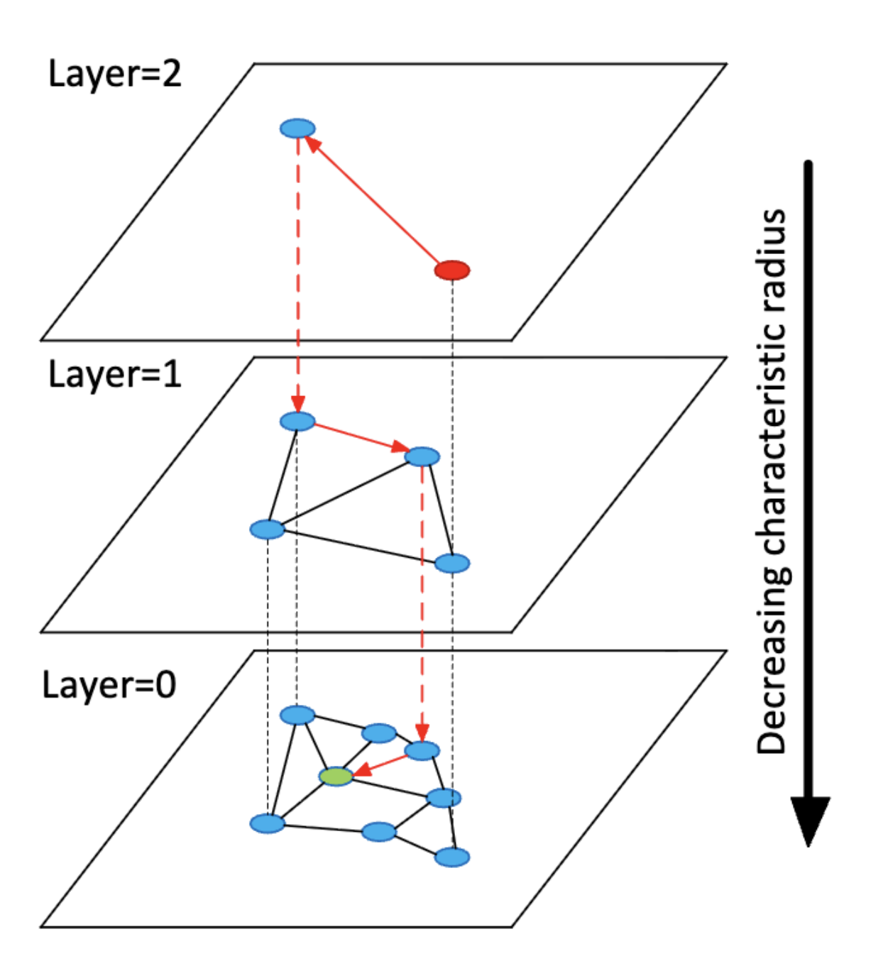
Stanford's HNSW slide, and below it the picture, enlarged. The picture comes from the HNSW paper.
Read the HNSW slide
In the picture, what are the red point, the red arrows, the red dashed arrows and the green point? How many steps are there from the red point to the green one?
Show the answer
The red point is the starting node on the top layer. The red arrows are greedy steps, and the red dashed arrows show where the search got stuck and dropped down a layer. According to the HNSW paper's caption, the green point is the query. There is one step on each layer, so 3 steps in all. The black dashed lines show that every node of an upper layer is also in every layer below it. (Step 5)
What does the arrow on the right, “Decreasing characteristic radius”, say?
Show the answer
Edges get shorter in the lower layers. The upper layers have few nodes, so the edges between them are long, and one step covers a lot of ground. In our example the jump was 40 on layer 2, 20 on layer 1 and 5 on layer 0. (Step 5)
In “~log N hops, high recall”, what is the base of the log? How much is it for 100 million vectors, and where does the high recall come from?
Show the answer
The slide gives no base, because changing the base only changes a fixed factor. With log2, 100 million gives about 27, and the number of layers for M = 16 is log16, about 6.64. The steps on each layer stay below a fixed number, and the layers grow like log N. For high recall, layer 0 runs the ef search. (Steps 5 and 9)
Stanford's second HNSW slide: how the graph is built. The word “backup” in the title means it is an extra slide in the lecture. Below it is the picture, enlarged, which also comes from the HNSW paper.
Read the graph-building slide
The slide says: “Pick its top layer at random: most nodes stay in layer 0, few reach the top”. With M = 16, how many of 100 million nodes reach layer 1, and how many reach the top?
Show the answer
The chance of reaching each next layer is 1/16. So 100 million ÷ 16 = 6,250,000 nodes reach layer 1, and about 6 reach layer 6. The other 15/16, about 94 million nodes, stay only in layer 0. (Step 9)
In the picture, the new green node sits at the edge of cluster 1. Which rule picks the “extra link” to e2, and what would happen without it?
Show the answer
The rule for choosing neighbors: a candidate is linked only if it is nearer to the new node than to every node already linked. The other candidates in cluster 1 are nearer to nodes already linked, so they are skipped, while e2 lies in a new direction and gets linked. Without it the greedy walk would get stuck at the edge of cluster 1, as it did at X in our example. (Step 9)
How does the M in “M nearest neighbors” affect memory and recall?
Show the answer
On layer 0 each node has up to 2M edges, at 4 bytes each. For M = 16 that is about 151 bytes per vector, or 15.1 GB for 100 million vectors. According to the HNSW paper, a larger M is better for high recall, but memory grows with it. (Step 9)
3 points from this lesson
Brute force costs O(N·d), with distances too. For vectors of length 1, distance² = 2 − 2 × dot product, so a distance index also does the job of MIPS.
IVF's centroids come from k-means, and its comparisons are K + nprobe × N ÷ K, smallest at K = √(nprobe × N). PQ's codebooks also come from k-means, and with a lookup table each vector's score takes 96 additions.
In HNSW, 1/M of the nodes reach each higher layer, so there are about log N layers. ef sets the recall, and the rule for choosing neighbors keeps edges between clusters so the greedy walk does not get trapped.
New terms in this lesson
Exact search (brute force)
Comparing with every vector to get the guaranteed top-k. For example, with 21 vectors, computing 21 distances.
Big-O, O(N·d)
How the cost grows as N or d grows. For example, in O(N·d), if N doubles, the cost doubles too.
Nearest neighbors
The vectors nearest to the query. For example, among the neighbors of the query 73, 75 comes first.
ANN
Approximate nearest neighbor search: looking at fewer vectors and finding the right neighbors most of the time. For example, finding 9 of the true top-10 gives recall 0.9.
Distance
The length of the difference between two vectors. For example, [0.8, 0.2] and [0.9, 0.1] differ by [0.1, −0.1], so the distance is √(0.01 + 0.01) = 0.14.
IVF
Inverted file index: splitting the vectors into clusters and looking only at the clusters near the query. For example, 11,000 comparisons for 1 million vectors.
nprobe
How many clusters IVF looks at. For example, with 1,000 clusters and nprobe = 10, only the vectors of 10 clusters are checked.
Product quantization (PQ)
Cutting a vector into pieces and storing, for each piece, the number of its nearest codeword. For example, [0.9, 0.1, 0.2, 0.8] becomes the code (0, 1).
Codebook
The list of sample vectors (codewords) for a piece. For example, #0 [1, 0], #1 [0, 1], #2 [0.5, 0.5], #3 [0.7, 0.7].
Proximity graph
A graph in which every vector is linked to its nearby vectors. For example, 70 is linked to its neighbors 65 and 75.
Greedy search
Moving at every step to the neighbor nearest to the query, until stuck. For example, moving from 70 to 75 for the query 73.
HNSW
A layered proximity graph: a greedy walk from the top, dropping one layer when stuck. For example, 4 steps for the query 73.
k-means
A way to split vectors into k clusters: give each vector to its nearest centroid, then make each centroid the average, and repeat. For example, on 6 passages it ends after 3 rounds with A = [0.817, 0.2] and B = [0.2, 0.8].
Lookup table (ADC)
Computing the score of every query piece with every codeword in advance and keeping them in a table. Each passage's score is then just a sum of table entries. For example, the score of code (0, 1) is 1 + 1 = 2.0.
Residual
What is left after subtracting a vector's cluster centroid from it. IVFADC stores the code of this difference. For example, queue log [0.85, 0.2] − [0.817, 0.2] = [0.033, 0].
ef
The size of the list of nearest nodes found so far in an HNSW search. A larger ef means more distances and higher recall. For example, starting at node 70 with ef = 3 gives {75, 70, 80}.
Rule for choosing neighbors (heuristic)
A candidate is linked only if it is nearer to the new node than to every node already linked. For example, X links to A and E2, and B and C are skipped.