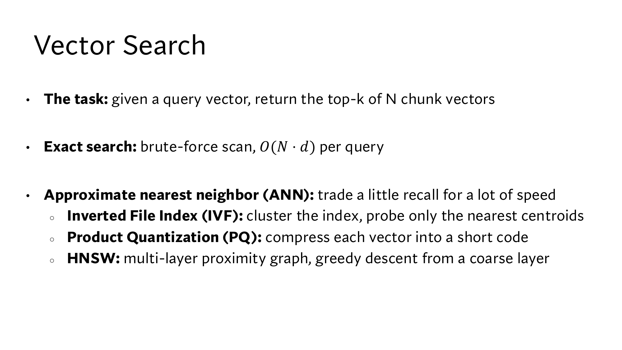
The job of vector search is to find the k vectors nearest to the query's vector. This lesson teaches methods that find those same k vectors most of the time without looking at every vector. The retriever in lesson 3 compared each query with every vector in the index. For the 60,000 passages of the company in lesson 2 that takes a moment, but on 100 million passages each query would take about 7.7 seconds. my estimate
The search in lesson 5 finds the k passages with the largest dot products, and the way to speed it up is the same: do not look at every vector. Then the nearest passage is sometimes missed, so this lesson also teaches you how to measure that miss.
The ladder for this lesson
The ladder has 5 steps. Under each step you can see what you will be able to do after it.
What you need first: Lesson 3 (vector, dot product, length) and Lesson 9 (cluster, centroid, graph). If you already know a step, skip to the next one. A word with a dotted underline and ▾ opens its definition when you click it.
1Comparing with every vector: exact search and its cost
Stanford's slide states the task of vector search like this: for a query vector, return the top-k of the N vectors in the index. The simplest method computes a score against every vector and returns the vectors with the k highest scores. This is called exact search, or brute force, because it looks at everything without any shortcut.
Its cost is easy to count. The of lesson 3's query [0.8, 0.2] with the office hours page [0.9, 0.1] is 0.8 × 0.9 + 0.2 × 0.1 = 0.74. That took 2 multiplications. Vectors with d numbers need d multiplications, so comparing with N vectors takes N × d multiplications.
Real vectors have a large d: a BERT-base vector has 768 numbers, so d = 768. For speed, take a rough estimate that a computer does 10 billion multiplications per second. my speed estimate
Corpus
Multiplications per query
Time per query
The company in lesson 260,000 passages
46 million60,000 × 768
0.005 second
Wikipedia in lesson 521 million passages
16.1 billion21 million × 768
1.6 seconds
A large corpus100 million passages
76.8 billion100 million × 768
7.7 seconds
The last row takes two steps:
Multiplications per query: 100 million × 768 = 76.8 billion.
Time: 76.8 billion ÷ 10 billion per second = 7.68 seconds, about 7.7 seconds.
The slide writes this cost as O(N·d), and this notation is called Big-O. Big-O does not give an exact count. It tells you how the cost grows as N or d grows. O(N·d) means that if N doubles, the cost doubles, and if d doubles, it also doubles. In the table N went from 60,000 to 100 million, about 1,667 times as many, and the time went from 0.005 to 7.7 seconds, the same factor.
Brute force always returns the true top-k, so on a small corpus it is the best method. The trouble is only on a large corpus, where each query takes seconds.
2ANN: give up a little recall for a lot of speed
Without looking at every vector you cannot be sure of the top-k, because the vector you skipped might be the nearest one. So on a large corpus you have to make a trade: look at fewer vectors, and get the right answer most of the time. The vectors nearest to a query are called its nearest neighbors.
ANN, approximate nearest neighbor search, is the family of methods that look at only a few vectors and still return the true nearest neighbors most of the time. Approximate means nearly. The slide calls it a trade: trade a little recall for a lot of speed.
Here means: of the true top-10 that brute force would return, how many did the ANN return? If the ANN returned 9 of the 10, the recall is 9 ÷ 10 = 0.9. A passage the ANN drops never reaches the reader. So this miss pushes down the from lesson 2.
Recall@k in lesson 13 is a different thing. There the right answer comes from human labels, and here it comes from brute force's top-10.
Distance: how to measure “near”
To measure “near”, the methods in this lesson use distance. To find the distance between two vectors, first subtract the numbers in the same positions, which gives a difference vector. Then take its , the calculation from lesson 3: square each number, add the squares, then take the square root.
For lesson 3's query [0.8, 0.2] and the office hours page [0.9, 0.1], this takes three steps:
Difference: [0.9 − 0.8, 0.1 − 0.2] = [0.1, −0.1].
Sum of squares: 0.1 × 0.1 + (−0.1) × (−0.1) = 0.01 + 0.01 = 0.02. The square of a negative number is positive too.
Square root: √0.02 = 0.14. Check: 0.14 × 0.14 = 0.0196, which is about 0.02.
The syllabus [0.1, 0.9] differs by [−0.7, 0.7], and its distance is √(0.49 + 0.49) = √0.98 = 0.99. The smaller the distance, the nearer the vector, so the office hours page is nearer to the query.
Stanford's slide: vector search. You can now read the first three lines: the task, the cost of exact search O(N·d), and the ANN trade. The three ANN methods below them, IVF, PQ and HNSW, come in the next three steps. Click the image to open it at full size.
3IVF: looking only at the clusters near the query
A query's nearest neighbors will be close to it, so looking at far-away vectors is wasted work. The difficulty is that you cannot tell a vector is far away without looking at it. Here the from lesson 9 helps, the average of a cluster's vectors. For example, the centroid of [0.1, 0.9], [0.2, 0.8] and [0.15, 0.85] is [0.15, 0.85]. If the query is far from a centroid, the vectors in its cluster are mostly far away too.
IVF (inverted file index) splits the vectors into clusters, and at search time looks only at the vectors in the clusters near the query. Its work has two parts:
: each vector goes into the cluster of its nearest centroid, and each centroid keeps a list of its vectors. These lists are called the inverted file.
Online: the query is first compared only with the centroids. IVF then picks a few of the nearest centroids and computes distances only to the vectors in their lists.
The number of clusters to look at is called nprobe. the name nprobe is not on the slide Suppose 1 million vectors are split into 1,000 clusters, about 1,000 vectors per cluster. With nprobe = 10, count the comparisons like this:
With the centroids: 1,000 comparisons.
With the vectors of the 10 chosen clusters: 10 × 1,000 = 10,000 comparisons.
11,000 in total, against 1,000,000 for brute force. 1,000,000 ÷ 11,000 = 91, so about 91 times less work.
Think first
The query sits at the edge between two clusters, and nprobe = 1. Will IVF find the true nearest point?
Show the answer
Not always. IVF looks only at the cluster whose centroid is nearest to the query. For a query at the edge, the nearest point can be in the neighbouring cluster. Pick “Query at the edge” in the widget and see.
Run IVF yourself
40 points, 4 clusters. The squares are centroids. Click the plane to place the query, and change nprobe. The dark points are the ones IVF looked at. The circled point is the true nearest one.
Pick “Query at the edge”. The centroid nearest to the query is the one on the right, so with nprobe = 1 IVF looks only at that cluster. That is 4 centroids and 11 points, 15 comparisons in total, against 40 for brute force. But the true nearest point is in the cluster on the left, and it is missed. With nprobe = 2 it is found, and the comparisons rise to 25.
This is the limit of IVF: when a query is at an edge, its nearest neighbors can be in the neighbouring cluster. “Query in the middle” even needs nprobe = 3. Raising nprobe raises recall and lowers speed, so the ANN trade is now set by a single number.
4PQ: turning each vector into a short code
IVF cut the comparisons, but all the vectors still have to sit in memory. A common number takes 4 bytes, so a vector of 768 numbers takes 768 × 4 = 3,072 bytes. 100 million vectors need 100 million × 3,072 = 307.2 billion bytes. A GB is 1 billion bytes, so that is 307 GB, about 300 GB. not on the slide
Product quantization (PQ) cuts each vector into pieces. It then replaces each piece with the number of the nearest vector in a fixed list. That list is called a codebook, and each vector in it a codeword. These numbers together make the vector's code, and the index stores this code instead of the real numbers. That is what quantization means: replacing a value with the nearest value from a fixed list.
Take the 4-number vector [0.9, 0.1, 0.2, 0.8] and cut it into two pieces: [0.9, 0.1] and [0.2, 0.8]. The codebook has 4 codewords: #0 [1, 0], #1 [0, 1], #2 [0.5, 0.5] and #3 [0.7, 0.7]. Here both pieces share one codebook, while real PQ has a separate codebook for each piece position. my example
Codeword
Distance from [0.9, 0.1]
Distance from [0.2, 0.8]
#0 [1, 0]
0.14
1.13
#1 [0, 1]
1.27
0.28
#2 [0.5, 0.5]
0.57
0.42
#3 [0.7, 0.7]
0.63
0.51
The first distance works out as [1 − 0.9, 0 − 0.1] = [0.1, −0.1], and √(0.01 + 0.01) = 0.14. The nearest codeword to the first piece is #0, and to the second piece #1. So the whole vector becomes just the code (0, 1).
From the code you can rebuild the vector roughly: #0 and #1 side by side give [1, 0, 0, 1]. Now look at the dot product with the query [1, 0, 0, 1]. With the real vector it is 1 × 0.9 + 0 × 0.1 + 0 × 0.2 + 1 × 0.8 = 1.7, and with the rebuilt vector it is 1 + 1 = 2.0.
At real scale, cut the 768 numbers into 96 pieces of 8, and give each codebook 256 codewords. A byte has 8 bits, and 8 bits make 2 × 2 × 2 × 2 × 2 × 2 × 2 × 2 = 256 different numbers. So every code from 0 to 255 fits in 1 byte, and the whole vector takes 96 bytes. common settings, not on the slide
The vector became 3,072 ÷ 96 = 32 times smaller, and 100 million vectors shrank from 300 GB to about 9.6 GB. The arithmetic: 100 million × 96 = 9.6 billion bytes, which is 9.6 GB.
The limit shows in the 1.7 and 2.0 above: a score from a code is an estimate, and close scores can swap order. That is why many systems score the last few candidates again with their real vectors.
Think first
With the codebook above, what is the code of the vector [0.65, 0.65, 0.95, 0.05]?
Show the answer
The nearest codeword to [0.65, 0.65] is #3 [0.7, 0.7], at distance 0.07. #2 [0.5, 0.5] is 0.21 away. The nearest to [0.95, 0.05] is #0 [1, 0], at distance 0.07. Code = (3, 0).
5HNSW: a greedy walk on a layered graph
IVF misses at the edges because it never looks at the vectors in the other clusters. A second idea builds no clusters at all: it connects each vector to a few of its nearby vectors. Such a graph is called a proximity graph, and every vector in it is a node, as in the graph from lesson 9.
A search on a proximity graph starts at one node, and at every step moves to the neighbor nearest to the query. When no neighbor is nearer than the current node, the search is stuck, and that node is the answer. This walk is called greedy search.
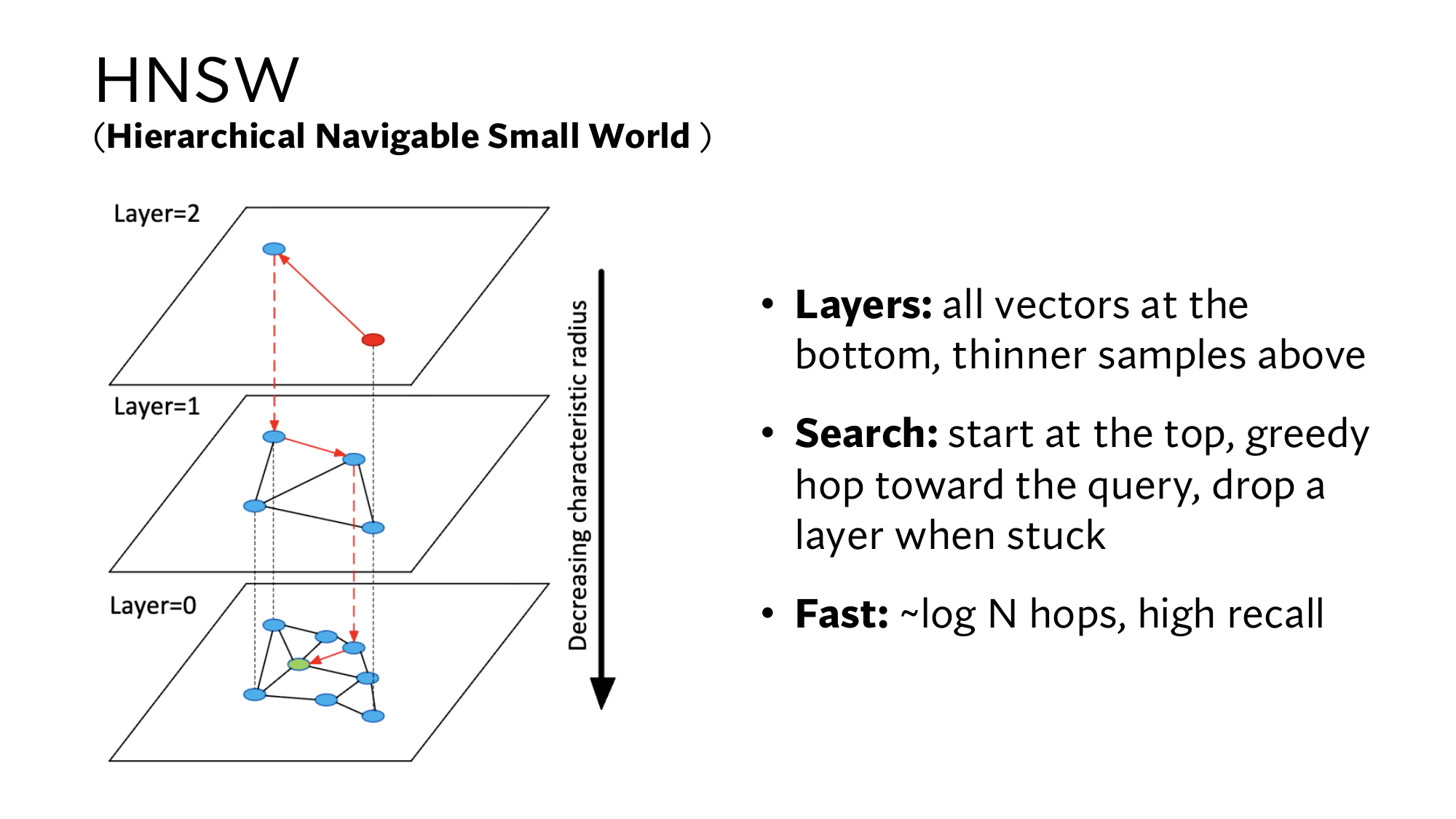
On a single layer, starting far away means many small steps. So HNSW (Hierarchical Navigable Small World) builds the graph in layers. Layer 0 holds every vector, and the layers above hold fewer nodes with longer jumps between them. The search starts at the top, and wherever it gets stuck, it drops down one layer.
So that you can do the arithmetic by hand, take a 1-dimensional example. The vectors are 21 numbers from 0 to 100, spaced 5 apart, and the distance is just the difference between two numbers. Each node is linked to its left and right neighbors in its layer. The query is 73, and the search starts at node 10 in layer 2. my example
Layer 2: 10, 50, 90
Layer 1: 10, 30, 50, 70, 90
Layer 0: 0, 5, 10, …, 100 (all 21)
Layer
At (distance)
Neighbors (distance)
Decision
2
10 (63)
50 (23)
Move to 50
2
50 (23)
10 (63), 90 (17)
Move to 90
2
90 (17)
50 (23)
Stuck, drop to layer 1
1
90 (17)
70 (3)
Move to 70
1
70 (3)
50 (23), 90 (17)
Stuck, drop to layer 0
0
70 (3)
?
?
0
75 (2)
70 (3), 80 (7)
Stuck. Answer: 75
Work out the sixth row
On layer 0 you are at node 70. Who are its neighbors, how far are they from the query 73, and what is the decision?
Show the answer
Layer 0 holds all 21 numbers, so 70's neighbors are 65 and 75. Distances: 65 (8) and 75 (2). 75 is nearer than the current node 70 (3), so move to 75.
It took 4 steps in total (50, 90, 70, 75), and the answer is right, because 75 is the nearest number to 73. Along the way the search computed the distance to 7 nodes, while brute force would compute all 21.
As N grows, this gap grows a lot. The slide says HNSW takes about steps, roughly the number of times you multiply 2 by itself to reach N. Multiplying 2 by itself 20 times gives 1,048,576. So 1 million vectors take about 20 steps, and 100 million about 27.
Stanford's slide: the layers of HNSW. The red point is the starting node at the top, the red arrows are the greedy walk, and the red dashed arrows show where the search dropped down a layer. The green point is the query. The arrow on the right says that edges get shorter in the lower layers, as in our example with jumps of 40, 20 and 5. Click the image to open it at full size.
The price of HNSW is memory, because every node also has to store its edges. not on the slide Its limit is that the greedy walk can get stuck at a node that is not the true nearest one. This happens especially when the vectors fall into separate groups. That is why HNSW also gives each new vector one edge to a different group.
What the dense version adds
The dense version contains this whole lesson, followed by 5 more steps that take you to the level of the Stanford slides:
Step 6: the maths of distance, and why distance and dot product give the same order for vectors of length 1.
Step 7: k-means for IVF's centroids, and how many clusters to make.
Step 8: PQ codebooks, fast scores from a lookup table, and PQ together with IVF.
Step 9: HNSW's random layers, ef, the rule for choosing neighbors, and memory.
Step 10: Stanford's three vector search slides, which you read yourself.
Brute force costs O(N·d): it is always right, but on 100 million passages each query takes about 7.7 seconds.
ANN looks at fewer vectors, and its recall tells you how many of the true top-k it found. IVF looks only at the nearby clusters, and nprobe sets the trade.
PQ turns each vector into a code of 96 bytes instead of 3,072. HNSW walks greedily down a layered graph, in about log N steps.
New terms in this lesson
Exact search (brute force)
Comparing with every vector to get the guaranteed top-k. For example, with 21 vectors, computing 21 distances.
Big-O, O(N·d)
How the cost grows as N or d grows. For example, in O(N·d), if N doubles, the cost doubles too.
Nearest neighbors
The vectors nearest to the query. For example, among the neighbors of the query 73, 75 comes first.
ANN
Approximate nearest neighbor search: looking at fewer vectors and finding the right neighbors most of the time. For example, finding 9 of the true top-10 gives recall 0.9.
Distance
The length of the difference between two vectors. For example, [0.8, 0.2] and [0.9, 0.1] differ by [0.1, −0.1], so the distance is √(0.01 + 0.01) = 0.14.
IVF
Inverted file index: splitting the vectors into clusters and looking only at the clusters near the query. For example, 11,000 comparisons for 1 million vectors.
nprobe
How many clusters IVF looks at. For example, with 1,000 clusters and nprobe = 10, only the vectors of 10 clusters are checked.
Product quantization (PQ)
Cutting a vector into pieces and storing, for each piece, the number of its nearest codeword. For example, [0.9, 0.1, 0.2, 0.8] becomes the code (0, 1).
Codebook
The list of sample vectors (codewords) for a piece. For example, #0 [1, 0], #1 [0, 1], #2 [0.5, 0.5], #3 [0.7, 0.7].
Proximity graph
A graph in which every vector is linked to its nearby vectors. For example, 70 is linked to its neighbors 65 and 75.
Greedy search
Moving at every step to the neighbor nearest to the query, until stuck. For example, moving from 70 to 75 for the query 73.
HNSW
A layered proximity graph: a greedy walk from the top, dropping one layer when stuck. For example, 4 steps for the query 73.