Questions spread across a whole document: RAPTOR and GraphRAG
RAPTOR and GraphRAG put summaries into the index next to the chunks, so that answers spread across a whole document can still be found. RAPTOR builds a tree of summaries, and GraphRAG builds a graph of the things in the text and how they relate.
You can see the need with this question: What are all the deadlines? The answer is 4 dates in the course, spread over three passages from lesson 2. The syllabus has the milestone (Week 6) and the final report (Week 10). The project page has the proposal (Oct 9), and the Homework 1 announcement has its release date (Oct 5). The retriever ranks the project page first, so with K = 1 the reader gets 1 of the 4 dates. from my vectors
The ladder for this lesson
The ladder has 10 steps. The first 5 are the same as in the easy version, and steps 6 to 10 take you to the level of the Stanford slides. Under each step you can see what you will be able to do after it.
What you need first: Lesson 3 (vector, cosine), Lesson 6 (indexing time, query time) and Lesson 7 (chunk, mean pooling). From step 6 on, Lesson 4 (exp, softmax, marginalization, likelihood) also helps. If you already know a step, skip to the next one. A word with a dotted underline and ▾ opens its definition when you click it.
1Top-K brings back only pieces
A detail question has its answer written in one passage, while the answer to a thematic question is built from several passages.When is the milestone due? is a detail question, because the answer is one line of the syllabus. What are all the deadlines? is thematic, because its 4 dates sit in three passages.
The retriever scores every passage on its own and returns the top K. For a thematic question, each passage holds only part of the answer. Below, every text has a vector of 4 numbers. The first number says how much the text is about the milestone, the second about the other deadlines, and the third about office hours. The fourth says how many things the text pulls together, that is, how much of an overview it is. my vectors
The milestone question's vector is [0.95, 0.2, 0, 0.05], and the all-deadlines question's is [0.4, 0.5, 0, 0.8].
is the measure from lesson 3: divide the dot product by the product of the two vectors' lengths. For the syllabus and the all-deadlines question it takes three steps:
On the detail question the syllabus gets 0.99, a clear win. On the thematic question the highest cosine is the project page's 0.66, and it holds 1 of the 4 dates. No passage is about “all the deadlines”, so none of them gets a high cosine. The question's fourth number is 0.8, because it asks for an overview, while every passage's fourth number is only 0.1 or 0.15.
Think first
How many dates does the reader get with K = 3? And if a 40-page syllabus had 10 deadlines in 10 separate chunks, how many would K = 3 bring?
Show the answer
Among these 6 passages the top 3 are the project page (0.66), the Homework 1 announcement (0.61) and the syllabus (0.60), so all four dates arrive. But in the 10-chunk syllabus, K = 3 leaves out at least 7 deadlines. K is fixed in advance, and the retriever does not know how many pieces a question needs. my example
One big chunk for the whole syllabus does not work either. In lesson 7 a big chunk's vector was the average of its topics, which is . There, mixing just two topics dropped the cosine from 1.00 to 0.71. So the index needs a text that is itself about all the deadlines, a written summary of several passages.
2Groups of similar passages: clustering
One summary of all 6 passages would be too coarse. A summary of the deadlines and a separate one of office hours are more useful. So before writing summaries, split the passages into groups by topic.
Clustering means splitting vectors into groups so that the vectors in a group are close to each other and far from the other groups. Each group is called a cluster. Here cosine is enough to measure “close”: the nearer the cosine is to 1, the more the two vectors point the same way.
To keep the arithmetic small, use the 2-number vectors from lesson 3. The first number says how much the text is about office hours, and the second how much it is about deadlines. my vectors
Pair
Cosine
Result
Syllabus [0.1, 0.9] and project page [0.2, 0.8]
0.99
Same cluster
Office hours page [0.9, 0.1] and queue log [0.85, 0.2]
0.99
Same cluster
Syllabus [0.1, 0.9] and office hours page [0.9, 0.1]
0.22
Different clusters
The first row works out like this. The dot product is 0.1 × 0.2 + 0.9 × 0.8 = 0.02 + 0.72 = 0.74. The lengths are √(0.01 + 0.81) = 0.906 and √(0.04 + 0.64) = 0.825, so the cosine is 0.74 ÷ (0.906 × 0.825) = 0.74 ÷ 0.747 = 0.99.
Compare the other pairs the same way and two clusters form. The deadlines cluster holds the syllabus, the project page and the Homework 1 announcement [0.15, 0.85]. The office hours cluster holds the office hours page, the queue log and the old forum post [0.8, 0.15].
Each cluster also has a middle point that can stand in for the whole cluster. The centroid is the average of the cluster's vectors, taken separately for each position. In the deadlines cluster the first number is (0.1 + 0.2 + 0.15) ÷ 3 = 0.15, and the second is (0.9 + 0.8 + 0.85) ÷ 3 = 0.85. So the centroid is [0.15, 0.85], and the office hours cluster's is [0.85, 0.15]. In lesson 10, centroids make search faster.
Some passages sit between two topics. The long FAQ page from lesson 3, [1.6, 1.4], has a cosine of 0.86 with the office hours centroid and 0.78 with the deadlines centroid. RAPTOR can put such a passage into both clusters, so that its content reaches both summaries. This is called soft clustering.
3RAPTOR: a tree of summaries, built bottom up
RAPTOR has an LLM write a summary of each cluster, and stores that summary in the index just like a chunk. The summary is new text, not an average of vectors. So its vector points towards “all the deadlines”, whereas the vector of lesson 7's big chunk got lost in the average.
Summaries can themselves be summarized: the deadlines summary and the office hours summary give one summary of the whole course. A structure with levels like this is called a tree. Each box in the tree is a node. The nodes at the bottom, the actual chunks, are called leaves, and the node at the top is the root.
RAPTOR stands for Recursive Abstractive Processing for Tree-Organized Retrieval, and Sarthi and colleagues at Stanford built it in 2024 from the paper. The tree is built bottom up in five steps:
Embed every chunk.
Cluster the embeddings.
Give each cluster's chunks to an LLM and have it write their summary. The summary is a new node one level up.
Embed the summaries.
Repeat steps 2 to 4 until only a handful of nodes are left at the top.
On the course corpus the tree looks like this. The 6 passages are the leaves, there are 2 summaries above them, and 1 root at the top. my example
Level
Node
Text
2, root
R, course overview
CS 329Z logistics: deadlines from Oct 5 to Week 10, and office hours on Tuesday and Thursday.
1
A, deadlines summary
Homework 1 releases Oct 5. Proposal due Oct 9. Milestone due Week 6, Thursday 11:59pm, no late days. Final report Week 10.
1
B, office hours summary
Tuesday 4pm in Room 104 (busy, about 14 waiting) and Thursday 9am on Zoom (about 3). An old 2024 post says midweek afternoons are quiet.
0, leaves
6 passages
The 6 passages from lesson 2
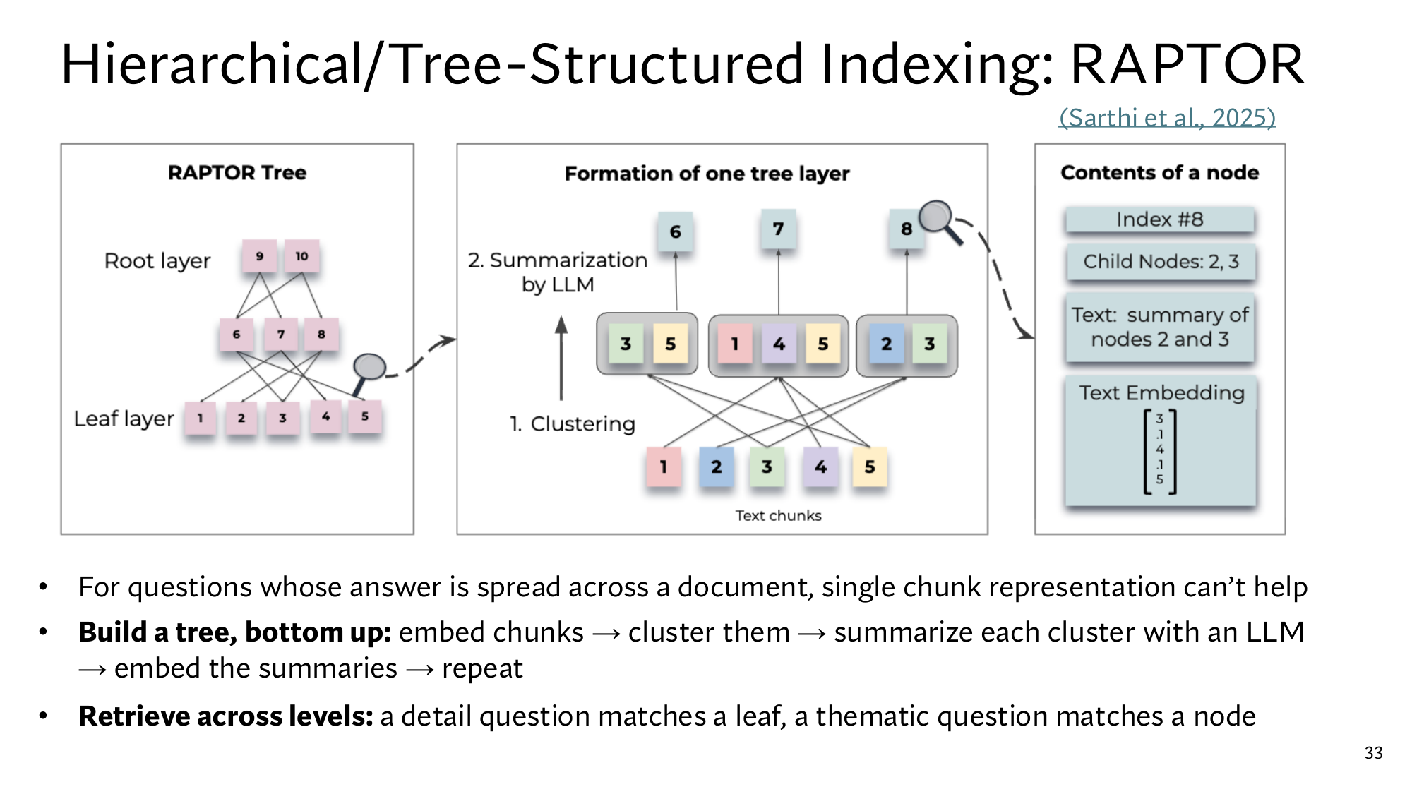
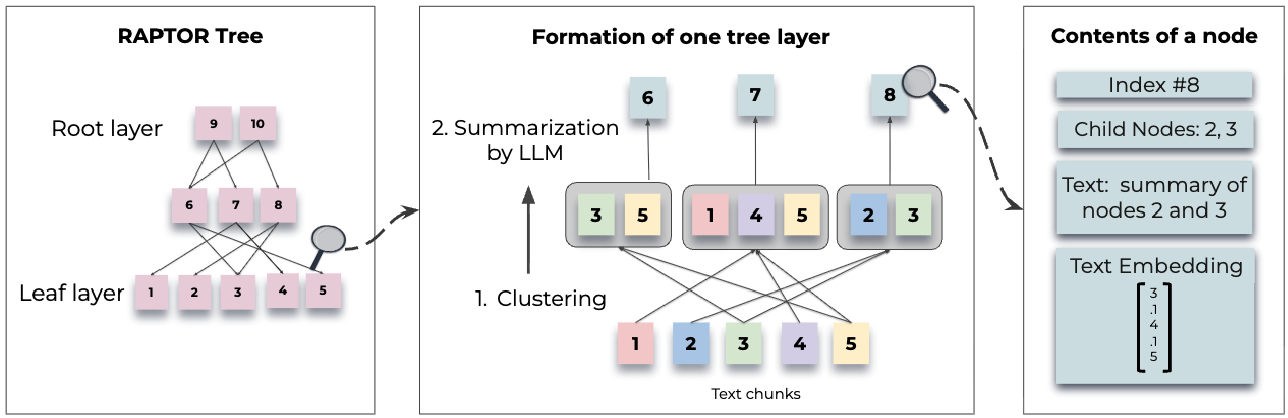
Stanford's RAPTOR slide: the whole tree on the left, the two steps that form one level in the middle, and the contents of one node on the right. Click the image to open it at full size.
In the middle box, 5 chunks form 3 groups: {3, 5}, {1, 4, 5} and {2, 3}. Chunks 3 and 5 are each in two groups, so this is soft clustering. Each group's summary becomes a node above: 6, 7 and 8. The right box shows node 8's children (2 and 3), their summary, and the embedding of that summary.
The cost comes at indexing time, because every cluster on every level needs one LLM call. An LLM writes the summaries, so it can drop a fine detail or get something wrong. Node B puts the old post's opinion on the same footing as the queue log's data. So the old forum post's problem now sits inside a summary.
Think first
A corpus has 64 chunks, and each cluster holds about 4 nodes. How many levels does it take to reach the root, and how many summaries are there in total?
Show the answer
Level 1 has 64 ÷ 4 = 16 summaries, level 2 has 16 ÷ 4 = 4, and level 3 has 4 ÷ 4 = 1 root. That is 16 + 4 + 1 = 21 summaries in total, so 21 LLM calls at indexing time. There are 3 levels above the leaves.
4Searching every level of the tree
RAPTOR matches the question against nodes on every level of the tree, the leaves and the summaries alike. Leaves and summaries sit in the same index, so the retriever computes a cosine for every node and returns the top ones. In the widget every node has a 4-number vector, and the summaries have a large fourth number, because they pull many things together. my vectors
Which level of the tree does a question match?
Pick a question. The table shows every node's cosine, highest first. Before you pick, guess which level's node the question will match.
Node
Level
Cosine
The milestone question matches the syllabus leaf at 0.99. The all-deadlines question matches summary A at 1.00, and A holds all four dates. In step 1 the best passage, the project page, reached only 0.66 and held 1 date. The overview question matches the root R. I made the vectors of A and R equal to the questions' vectors, so their cosine is exactly 1.00. With real embeddings it would be below 1.
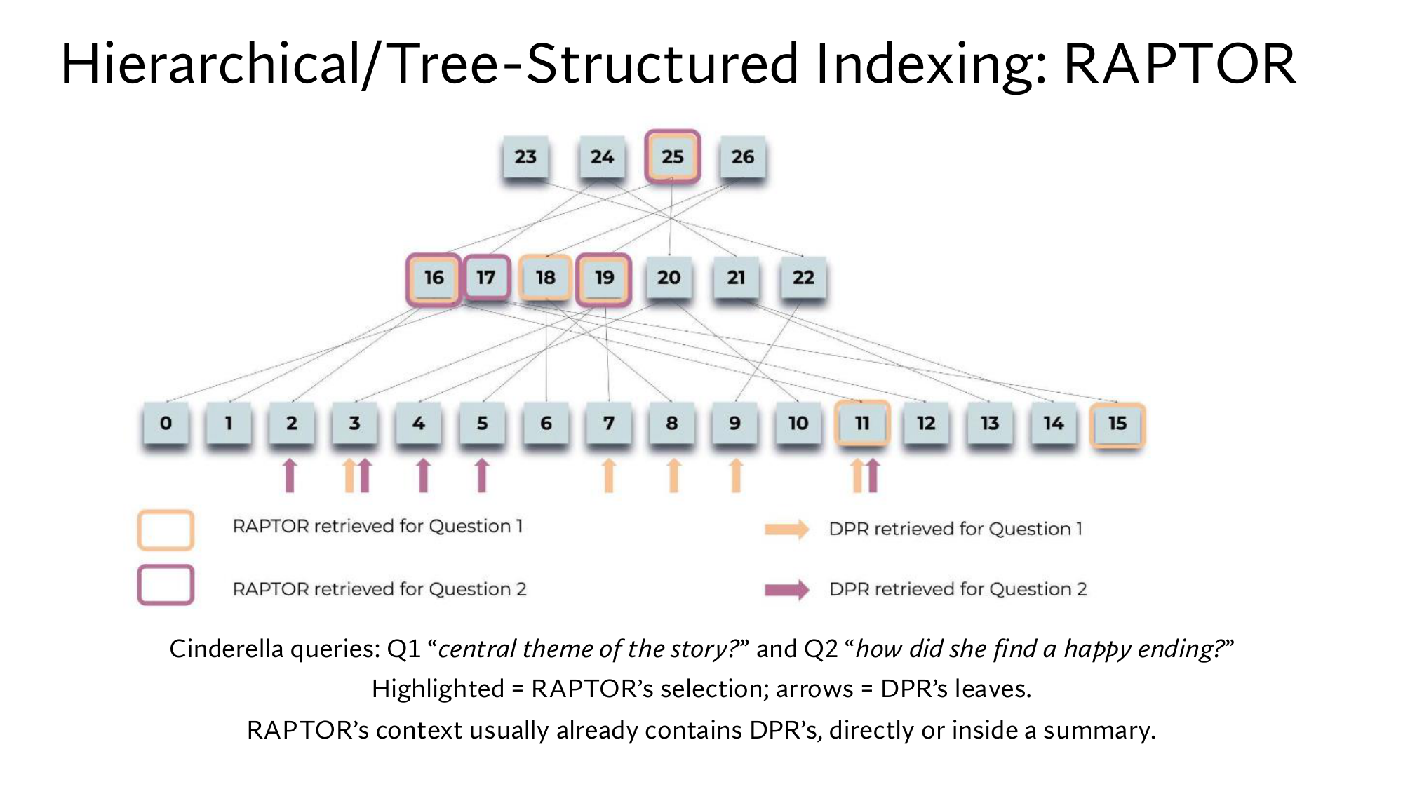
Stanford's slide says the same in one line: a detail question matches a leaf, and a thematic question matches a node higher up. The RAPTOR paper showed this with two questions about the Cinderella story: central theme of the story? and how did she find a happy ending?
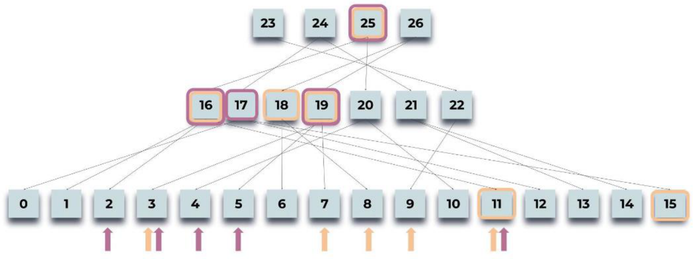
Stanford's Cinderella slide. Boxes with a coloured border are the nodes RAPTOR chose, and the arrows at the bottom mark the leaves DPR chose. Orange is the first question, and purple the second.
, the retriever in the RAG model of lesson 5, searches only the leaves. RAPTOR chose nodes from the upper levels too, for both questions. According to the slide, what DPR's leaves say is usually already in RAPTOR's context, either directly or inside a summary.
5GraphRAG: a graph of things and relations
RAPTOR forms its groups by how close the vectors are. But documents also state relations between things outright: the milestone is due in Week 6, and the TAs run office hours. GraphRAG forms its groups from these relations, and answers questions about the whole corpus from each group's summary.
Any named thing is called an entity: a person, a place, a course, a document or a date. Examples are Project milestone, Week 6, TAs and Room 104. A link between two entities is called a relation, and it is written in three parts: (entity, relation, entity). For example, (Project milestone, due, Week 6).
In GraphRAG an LLM reads every chunk and pulls out these relations. The course corpus gives these 7 rows: my example
Entity
Relation
Entity
Project
has part
Proposal, Project milestone, Final report
Proposal
due
Oct 9
Project milestone
due
Week 6
Final report
due
Week 10
Homework 1
released
Oct 5
Office hours
run by
TAs
Office hours
held in
Room 104, Zoom
Now make every entity a node, and every relation a line between two nodes. These lines are called edges, and a network of nodes and edges is a graph. A graph of entities and relations is called a knowledge graph. From the first row, Project links to three nodes, and each part links to its date.
In some parts of a graph the nodes are tightly linked to each other and only loosely to the rest. Such a part is called a community. Our graph has three communities, and no edge links them to each other. The first holds Project, its three parts and their dates. The second holds Office hours, TAs, Room 104 and Zoom, and the third holds Homework 1 and Oct 5.
Edge and colleagues at Microsoft Research built GraphRAG in 2024 from the paper. It has five steps at indexing time and two at query time:
Indexing time
Query time
1. Split the documents into chunks. 2. An LLM pulls entities and relations out of every chunk. 3. Build the knowledge graph from them. 4. Find the communities in the graph. 5. An LLM writes a summary of each community.
6. From each community's summary, an LLM writes a partial answer to the question. 7. An LLM combines all the partial answers into one global answer.
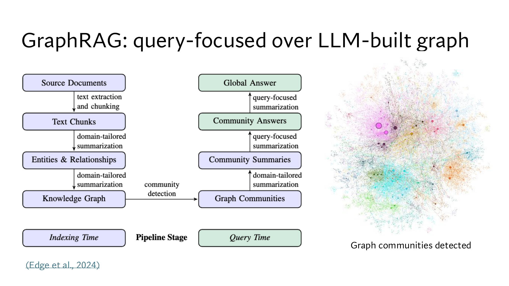
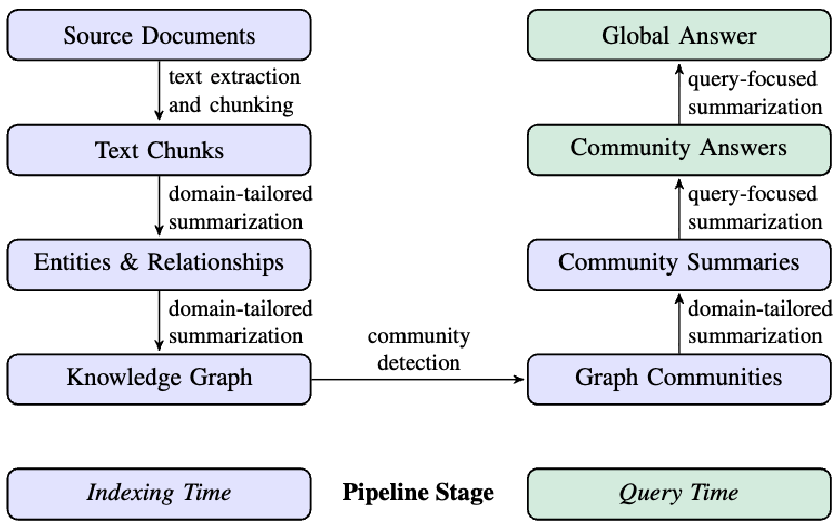
Stanford's GraphRAG slide. The indexing steps run down the left, and the query steps run up the middle. On the far right is a real graph, where each colour is one community.
For our question, step 6 writes one partial answer per community. The Project community gives three dates, the Homework 1 community gives one, and the office hours community gives none. Step 7 combines them into an answer with all four dates.
In steps 6 and 7 the LLM writes its summary with the question in mind, which is called query-focused summarization. The slide's title uses exactly this term. RAPTOR's summaries are written before any question arrives, while GraphRAG's final summary is written when the question arrives.
GraphRAG pays off on global questions about the whole corpus, where top-K passages do not work at all. The cost is high: LLM calls for every chunk and every community at indexing time, and one call per community at query time too. If the LLM extracts a wrong entity or relation, the mistake settles in the graph and reaches that community's summary.
Think first
Your company has 2,000 support tickets. Two questions come in: (a) Which product is ticket #4471 about? (b) What do customers complain about most? For which one is plain top-K enough, and for which is it not?
Show the answer
(a) is a detail question, because its answer is written in one ticket, so top-K is enough. (b) is thematic, because the answer comes from combining hundreds of tickets, and no single ticket will score high. It needs summaries, and since the question covers the whole corpus, GraphRAG fits.
From here: the Stanford level
The 5 steps above are the same as in the easy version. The 5 steps below take you to the level of the Stanford slides: first the maths of RAPTOR's clustering, then the methods and results of the RAPTOR and GraphRAG papers, then the whole GraphRAG family, and finally reading the slides yourself. Every piece of maths is explained where it first appears.
6The maths of RAPTOR's clustering: the Gaussian mixture and soft membership
In step 2 the clusters were formed by hand from cosines, and the FAQ page went into both. RAPTOR makes this decision with a probability model called a Gaussian mixture model (GMM) from the paper. The model gives every passage a probability for every cluster, and soft clustering runs on that probability. We build it in four moves: distance, the bell curve of one cluster, the mixture of several curves, and membership.
Distance: how far from the centroid
A GMM looks at instead of cosine. The distance between two vectors is the length of their difference: square each number of the difference, add them up, and take the square root. The old forum post is [0.8, 0.15], and the office hours centroid is [0.85, 0.15]. The difference is [−0.05, 0], so the distance is √(0.0025 + 0) = 0.05.
From the deadlines centroid [0.15, 0.85] the difference is [0.65, −0.7], and the distance is √(0.4225 + 0.49) = √0.9125 = 0.955. So the forum post sits very close to the office hours centroid, and about 19 times as far from the deadlines one.
One cluster: a bell curve
A GMM treats each cluster as a bell curve that is highest at the centroid and falls quickly as you move away. This curve is called a Gaussian. Its height follows e−d²/(2σ²), where d is the distance from the centroid. σ (sigma) is the cluster's spread, how far its points usually lie from the centroid, and it is called the .
A negative power of e is smaller than 1, because e−a = 1 ÷ ea. In lesson 4, (−1) = 1 ÷ 2.718 = 0.368. So the further the distance, the faster the height falls:
Distance d from the centroid
d²/(2σ²)
Height e−d²/(2σ²)
0
0
1.000
σ
0.5
0.607
2σ
2
0.135
3σ
4.5
0.011
For data with one number, the full Gaussian formula is this, where x is the point and μ (mu) is the middle of the curve:
𝒩(x; μ, σ) = 1σ√(2π) e−(x − μ)²/(2σ²)
The factor 1 ÷ (σ√(2π)) in front only makes the total area under the curve equal 1. With μ = 0 and σ = 1, the height is 0.399 at x = 0, 0.242 at x = 1 and 0.054 at x = 2. Check: 0.242 ÷ 0.399 = 0.607, the second row of the table. This height is not a probability. It is called a density, and for a narrow curve it can go above 1.
For a vector with two numbers, (x − μ)² is replaced by d², the squared distance from the centroid, and the factor in front becomes 1 ÷ (2πσ²). Here I assume the spread is the same in every direction, and that both clusters have σ = 0.25 my choice of σ. Then 2σ² = 0.125, and the factor in front is 1 ÷ (2π × 0.0625) = 2.546.
Several clusters: the mixture
A Gaussian mixture is a weighted sum of several bell curves. Each cluster k has a weight πk, the share of all passages that belong to it. Our 6 passages split 3 and 3, so both weights are 0.5, and the height of the mixture at a point x is:
This is the from lesson 4: each case's weight times that case's probability, then add them all, as in 0.5 × 0.8 + 0.5 × 0.1 = 0.45. There the cases were days, and here the cases are clusters. The paper writes the same thing for K clusters:
P(x) = ∑k=1K πk 𝒩(x; μk, Σk)
In our example K = 2, both πk are 0.5, and the μk are the two centroids, [0.85, 0.15] and [0.15, 0.85]. Here Σk is not the summation sign. It is the spread of cluster k, which can differ from direction to direction. In our simplification it is σ² = 0.0625 in every direction.
Soft membership: a probability for each cluster
Now take a new passage that mixes both topics: In milestone week, the Thursday office hours will run longer. Its vector is [0.6, 0.4] my passage. Membership is the probability that this passage came from cluster k. To get it, multiply the cluster's height by its weight, and divide by the total height P(x). In lesson 4, p(Tuesday | full) = 0.40 ÷ 0.45 = 0.89 came out exactly this way.
Squared distances: from the office hours centroid, (0.6 − 0.85)² + (0.4 − 0.15)² = 0.0625 + 0.0625 = 0.125, and from the deadlines one, (0.6 − 0.15)² + (0.4 − 0.85)² = 0.2025 + 0.2025 = 0.405.
Heights: e−0.125/0.125 = e−1 = 0.368, and e−0.405/0.125 = e−3.24 = 0.0392. Multiplying by 2.546 gives 𝒩office hours = 0.937 and 𝒩deadlines = 0.0997.
Times the weights: 0.5 × 0.937 = 0.468 and 0.5 × 0.0997 = 0.0499. The sum P(x) is 0.518.
Membership: office hours 0.468 ÷ 0.518 = 0.904, and deadlines 0.0499 ÷ 0.518 = 0.096. The two add up to 1.
p(k | x) = πk 𝒩(x; μk, Σk)∑j πj 𝒩(x; μj, Σj)
The top is the 0.468 from step 3, and the bottom is the sum 0.518. The 2.546 and the 0.5 appear on both top and bottom, so they cancel in the division. What remains is just the of e−1 and e−3.24: 0.368 ÷ (0.368 + 0.0392) = 0.904.
In RAPTOR's code a passage joins every cluster where its membership is above 0.1 from the RAPTOR code. Our passage's deadlines membership is 0.096, which is below 0.1. So it joins only the office hours cluster.
Think first
Lesson 7's big chunk [0.5, 0.5] was an equal average of office hours and deadlines. What are its two memberships, and how many clusters does it join?
Show the answer
Its squared distance from both centroids is (0.35)² + (0.35)² = 0.245, so both heights are the same: e−1.96 = 0.141. The memberships are 0.5 and 0.5, both above 0.1, so the chunk joins both clusters. (Steps 2 and 6)
I chose σ = 0.25 so the numbers stay readable. A real GMM works out μ, σ and π from the data itself, using a method called Expectation-Maximization (EM) from the paper. EM first computes every passage's memberships, then uses them to recompute the centroids, spreads and weights. It alternates these two moves until the numbers settle.
On our 6 points such a fit gives about σ = 0.04, because the points in each cluster are very close together my arithmetic. With σ that small, most memberships are almost exactly 0 or 1, and only passages right in the middle get split.
How many clusters: choosing with BIC
A GMM has to be told how many clusters there are. RAPTOR picks the count with BIC (the Bayesian Information Criterion): try several counts and keep the one with the smallest BIC from the paper. The paper's formula is:
BIC = ln(N) · k − 2 ln(L̂)
N is the number of passages, here 6, and ln 6 = 1.792. L̂ is the of the best fit, the product of every passage's P(x). Lesson 4's rule ln(a × b) = ln a + ln b turns that product into a sum. k is the number of model parameters, the numbers the fit decides.
In our simplified model each centroid has 2 numbers, and all clusters share one σ. K clusters have K − 1 weights, because the last weight is fixed by the others. my arithmetic
Clusters K
ln L̂
k, and ln(6) · k
BIC
1: all passages together
−4.51
3, 5.38
14.40
2: deadlines and office hours
17.20
6, 10.75
−23.64
3: office hours page on its own
18.12
9, 16.13
−20.11
The K = 2 row works out like this. In each passage's P(x) the other cluster's part is almost 0, so ln P(x) = ln 0.5 + ln 𝒩. The fit's σ² is 0.001667, and the squared distances add up to 0.02.
ln L̂ is positive here because the densities of narrow curves are above 1. At K = 3, ln L̂ rises only from 17.20 to 18.12, but the parameter penalty grows from 10.75 to 16.13. So BIC is smallest at K = 2, and RAPTOR would pick that count.
UMAP: shrinking the vectors first
The paper points out one more problem: in vectors with very many numbers, distance stops telling points apart well from the paper. To see this, I took 200 random points, each number between 0 and 1. Then I measured the distance from a random query to the nearest and the farthest point: my random points
Numbers per vector
Nearest, farthest
Farthest ÷ nearest
2
0.03, 0.80
25.94
10
0.58, 1.79
3.09
768
10.82, 12.07
1.11
With 768 numbers the nearest and the farthest point are almost equally far away, so “close” loses its meaning. That is why RAPTOR runs UMAP before clustering. UMAP turns each vector into one with far fewer numbers, and tries to keep points that were close before close in the new vectors. In RAPTOR's code the new vectors have 10 numbers from the RAPTOR code.
UMAP's n_neighbors sets how many neighbours each point looks at to decide its place. A large n_neighbors keeps the rough shape of the whole data, and a small one keeps the fine detail nearby. RAPTOR first forms rough global clusters, then local clusters inside each global one. If a cluster's text is longer than the summary model's token limit, RAPTOR clusters again inside it. from the paper
7The RAPTOR paper: two ways to search the tree, the setup and the results
Tree traversal and the collapsed tree
The paper tries two ways of searching the tree from the paper. Tree traversal works top down. From the top level, pick the k nodes closest to the question, then the k closest among only their children, and so on down to the leaves. The collapsed tree turns the whole tree into one list and sorts all nodes by cosine. It then adds nodes from the top until a token limit is full.
On our tree, traversal with k = 1 runs like this for the all-deadlines question. The root R is alone, so traversal starts there. Among its children, A (1.00) beats B (0.62). Among A's children, the project page (0.66) beats Homework (0.61) and the syllabus (0.60). The context is R, A and the project page.
The collapsed tree needs each node's token count, and we set the limit at 100 tokens: my token counts
Node, in cosine order
Cosine
Tokens, and running total
A, deadlines summary
1.00
30, 30
R, course overview
0.89
25, 55
Project page
0.66
15, 70
B, office hours summary
0.62
35, skipped (would be 105)
Homework 1 announcement
0.61
10, 80
Syllabus
0.60
20, 100
The difference shows on a detail question. On the milestone question, traversal takes one node per level: R (0.33), A (0.52), and then the syllabus (0.99). The collapsed tree puts the syllabus first. In traversal the mix of levels is the same for every question, while the collapsed tree picks the level to suit the question. The paper tried both on 20 QASPER stories, and the collapsed tree did better in every setting.
For its main experiments RAPTOR runs the collapsed tree with a limit of 2,000 tokens, which is about the top 20 nodes. The UnifiedQA reader reads only 512 tokens at a time, so it gets 400 tokens of context. The baselines get the same number of tokens. from the paper
How the tree was built
The paper's setup: from the paper
Chunks are 100 tokens long. If a sentence would cross the 100-token limit, the whole sentence moves to the next chunk instead of being cut.
Embeddings come from SBERT, a BERT-based encoder (multi-qa-mpnet-base-cos-v1).
gpt-3.5-turbo writes the summaries, with the prompt Write a summary of the following, including as many key details as possible.
A parent has 6.7 children on average, and a summary is about 0.28 times as long as its children's text combined, so 72% shorter.
The authors checked 150 nodes by hand and found a minor hallucination in 6 of them, which is 4%. These errors did not spread to the summaries above, and showed no effect on the answers.
Both the tokens and the time needed to build the tree grow in a straight line with the document's length.
Results on three datasets
The paper measures on three datasets. NarrativeQA has questions about books and movie scripts, 1,572 documents in all. QASPER has 5,049 questions about 1,585 NLP papers, and QuALITY has multiple-choice questions about passages of about 5,000 tokens. from the paper
QASPER is scored with F1, which compares the words of the reader's answer with the words of the right answer. Say the answer has 4 words, the right answer has 5, and 3 words appear in both my numbers. is 3 ÷ 4 = 0.75, and is 3 ÷ 5 = 0.6. F1 = 2 × 0.75 × 0.6 ÷ (0.75 + 0.6) = 0.9 ÷ 1.35 = 0.667, written as a percentage.
Retriever
GPT-3
GPT-4
UnifiedQA
BM25
46.6
50.2
26.4
DPR
51.3
53.0
32.1
RAPTOR
53.1
55.7
36.6
F1 (%) on QASPER. The columns are the reader that writes the answer, and the rows are the retriever. from the paper
RAPTOR leads with all three readers: by 1.8, 2.7 and 4.5 points over DPR, and by 6.5, 5.5 and 10.2 points over BM25. On QuALITY with GPT-3, accuracy is 57.3% for BM25, 60.4% for DPR and 62.4% for RAPTOR. RAPTOR helps every retriever: with UnifiedQA on QuALITY, BM25 goes from 49.9 to 52.1, and DPR from 53.1 to 54.7. from the paper
Paired with GPT-4, RAPTOR reaches 82.6% accuracy on QuALITY, against a previous best of 62.3%, so 20.3 points higher. On the HARD subset, the hardest questions, it is 76.2 against 54.7, so 21.5 points. On QASPER, RAPTOR with GPT-4 reaches an F1 of 55.7, 1.8 above the previous best of 53.9. from the paper
Which levels helped
On one QuALITY story the paper limited the search to different levels. Searching only the leaves gave 57.9% accuracy, and searching all three levels gave 73.68%. Of the nodes the collapsed tree returned, between 18.5% and 57% were not leaves but summaries from higher up, depending on the dataset and the retriever. from the paper
The paper also measured how much the clustering itself helps. Summarizing runs of 7 neighbouring chunks instead of clusters gave 55.8% accuracy on QuALITY. With GMM clustering it was 56.6%, a difference of 0.8 points. On Cinderella, GPT-4 given DPR's context said the happy ending could not be determined. Given RAPTOR's context, it answered correctly. from the paper
8The GraphRAG paper: building the graph, the map-reduce answer and the results
From chunks to a graph
GraphRAG splits documents into chunks of 600 tokens with a 100-token from the paper. So each new chunk brings 500 new tokens. Chunk size is a trade-off: larger chunks need fewer LLM calls, but the LLM misses entities in them. On HotPotQA data, GPT-4 found almost twice as many entity references in 600-token chunks as in 2,400-token chunks.
So GraphRAG gives the LLM a second pass, called gleaning. After extraction, GraphRAG asks the LLM a yes-or-no question: were any entities missed? If yes, the next prompt says many entities were missed, and the LLM extracts more. GraphRAG repeats this up to a set number of times. from the paper
The LLM also writes a short description for every entity and relation. It extracts claims as well, factual statements such as dates or events. When the same entity comes out of several chunks, it becomes one node, and the LLM summarizes its descriptions. The more times a relation is extracted, the higher its edge weight. If (Office hours, run by, TAs) came out of two passages, that edge would have weight 2.
Levels of communities: Leiden
To find communities, GraphRAG runs the Leiden algorithm from the paper. Leiden splits a graph into parts with many edges inside and few edges between them. GraphRAG runs it again and again: first communities, then sub-communities inside each community, until nothing can be split further.
This gives levels of communities: C0 is the top level, with the fewest communities, and C3 the bottom, with the most. On each level every node is in exactly one community. Here GraphRAG differs from RAPTOR, where one passage could sit in two clusters. Our graph would have three communities at level 0. At a lower level the Project community could split into a proposal part and a milestone part.
When writing a community's summary, the LLM's token limit can fill up, so GraphRAG puts the important parts first. A node's degree is the number of edges on it, and an edge's importance is the sum of its two nodes' degrees. In our graph Project has degree 3 and Proposal has degree 2. So (Project, has part, Proposal) has importance 3 + 2 = 5, and (Proposal, due, Oct 9) has 2 + 1 = 3. The edges with 5 go into the summary first.
When a question arrives: map-reduce
At query time GraphRAG writes its answer with map-reduce. Map means doing the same job on each piece separately, and reduce means combining all the results. In the paper this takes three steps: from the paper
Shuffle the community summaries of the chosen level, and split them into pieces of a fixed number of tokens.
Map: from each piece the LLM writes a partial answer. It also gives a score from 0 to 100 for how helpful the answer is, and parts that score 0 are dropped.
Reduce: the remaining parts are added in score order until the context window is full, and the LLM writes the final answer from them.
For our question, the Project part scores 95, the Homework 1 part 80, and the office hours part 0 my scores. The office hours part is dropped, and the reduce step reads the Project part, then the Homework 1 part, and writes all four dates. The paper used an 8k-token window for the summaries, the partial answers and the final answer.
Results from an LLM judge
Global questions have no single right answer, so the paper had an LLM write the questions too. For each dataset the LLM imagined 5 kinds of users, and 5 tasks for each user. Each task got 5 questions, so 5 × 5 × 5 = 125 questions. An example from a tech journalist: Which episodes deal primarily with tech policy and government regulation?from the paper
The paper used two datasets. The podcast transcripts were 1,669 chunks of 600 tokens (about 1 million tokens), and the news articles 3,197 chunks (about 1.7 million tokens). The graph built from the podcasts had 8,564 nodes and 20,691 edges, and indexing it with gpt-4-turbo took 281 minutes. from the paper
A second LLM then acted as the judge. It got a question and two systems' answers, and said for each criterion which answer was better, or that they were equal. There were four criteria: comprehensiveness (how much it covers), diversity (how many different angles), empowerment (how well the reader can understand and decide), and directness (how direct the answer is). The paper kept directness on purpose, as a check on the other results. It is the opposite of comprehensiveness, so no method can win on all four criteria.
Each pair was compared 5 times on every question, which gives 125 × 5 = 625 judgments. The win rate is the percentage of these in which the judge preferred one system, and 50% means a tie. A 72% win rate, for example, means about 0.72 × 625 = 450 judgments my arithmetic.
The paper compared six methods: the four community levels C0 to C3, TS and SS. TS runs the same map-reduce directly on the chunks, without a graph, and SS is ordinary vector RAG, which takes the closest chunks. On comprehensiveness, the global methods (the graph levels and TS) had win rates over SS of 72% to 83% on the podcasts and 72% to 80% on the news. On diversity they were 75% to 82% and 62% to 71%. On directness SS won, as expected. from the paper
The token cost differs too. The table shows how much context was read to answer each question on the podcasts: from the paper
Answered from
Units
Tokens per question
C0, the top communities
34
26,657
C1
367
225,756
C2
969
565,720
C3, the bottom communities
1,310
746,100
TS, the chunks directly
1,669
1,014,611
C0 needs only 26,657 ÷ 1,014,611 = 2.6% of TS's tokens, about 38 times fewer. On the news it is 39,770 ÷ 1,707,694 = 2.3%, about 43 times fewer. Even with so few tokens, C0 kept a 72% comprehensiveness win rate and a 62% diversity win rate over SS. from the paper
RAPTOR
GraphRAG
How groups form
By closeness of vectors (GMM), one passage can be in several clusters
From written relations (Leiden), each node in one community
When summaries are written
At indexing time
At indexing time, and again when the question arrives
Good for
Detail and thematic questions, from one index
Global questions about the whole corpus
9The whole GraphRAG family: the survey by Han and colleagues
Edge's GraphRAG is one system, but the name is now also used for a whole family. The 2025 survey by Han and colleagues calls any RAG whose data source is a graph a GraphRAG from the paper. Stanford's last GraphRAG slide comes from this survey, and you read it in step 10.
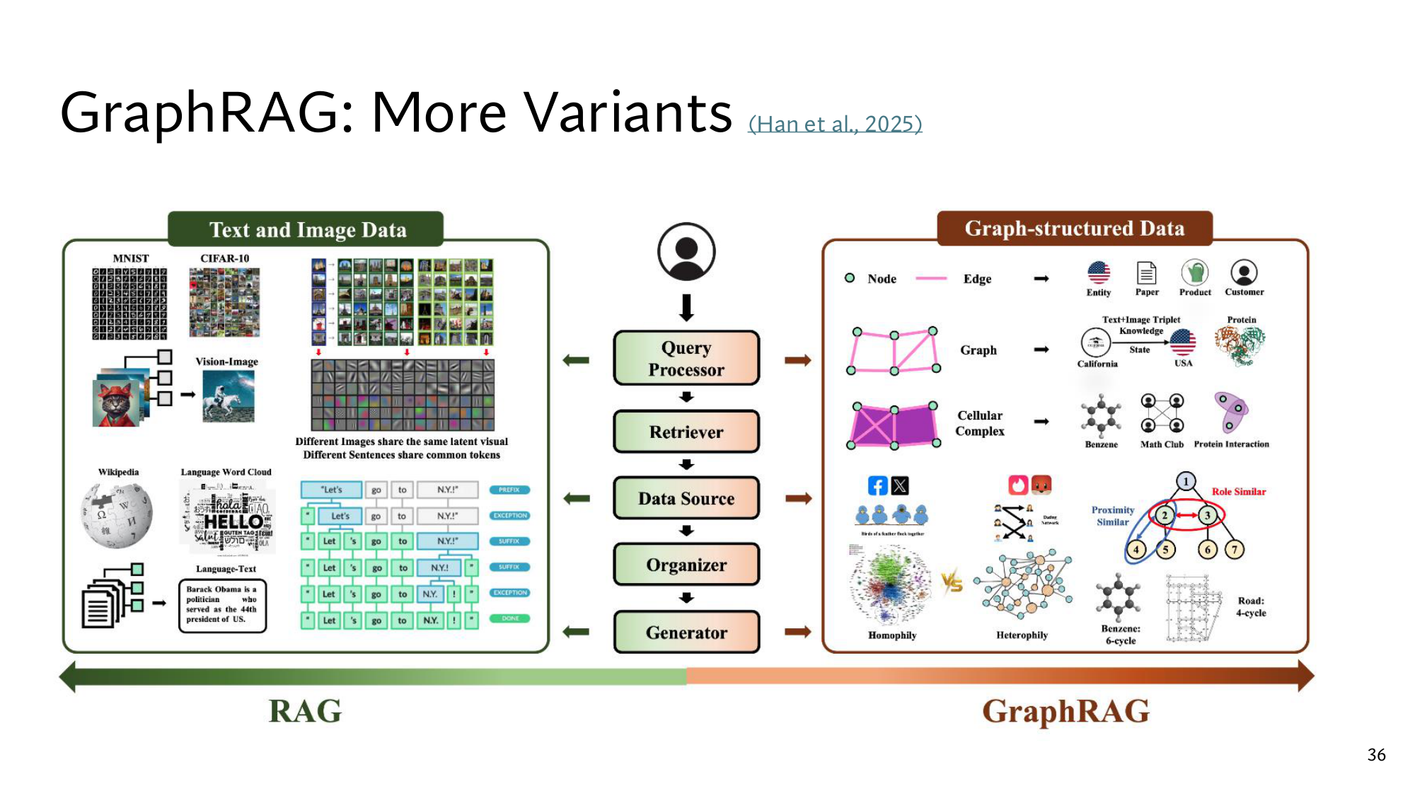
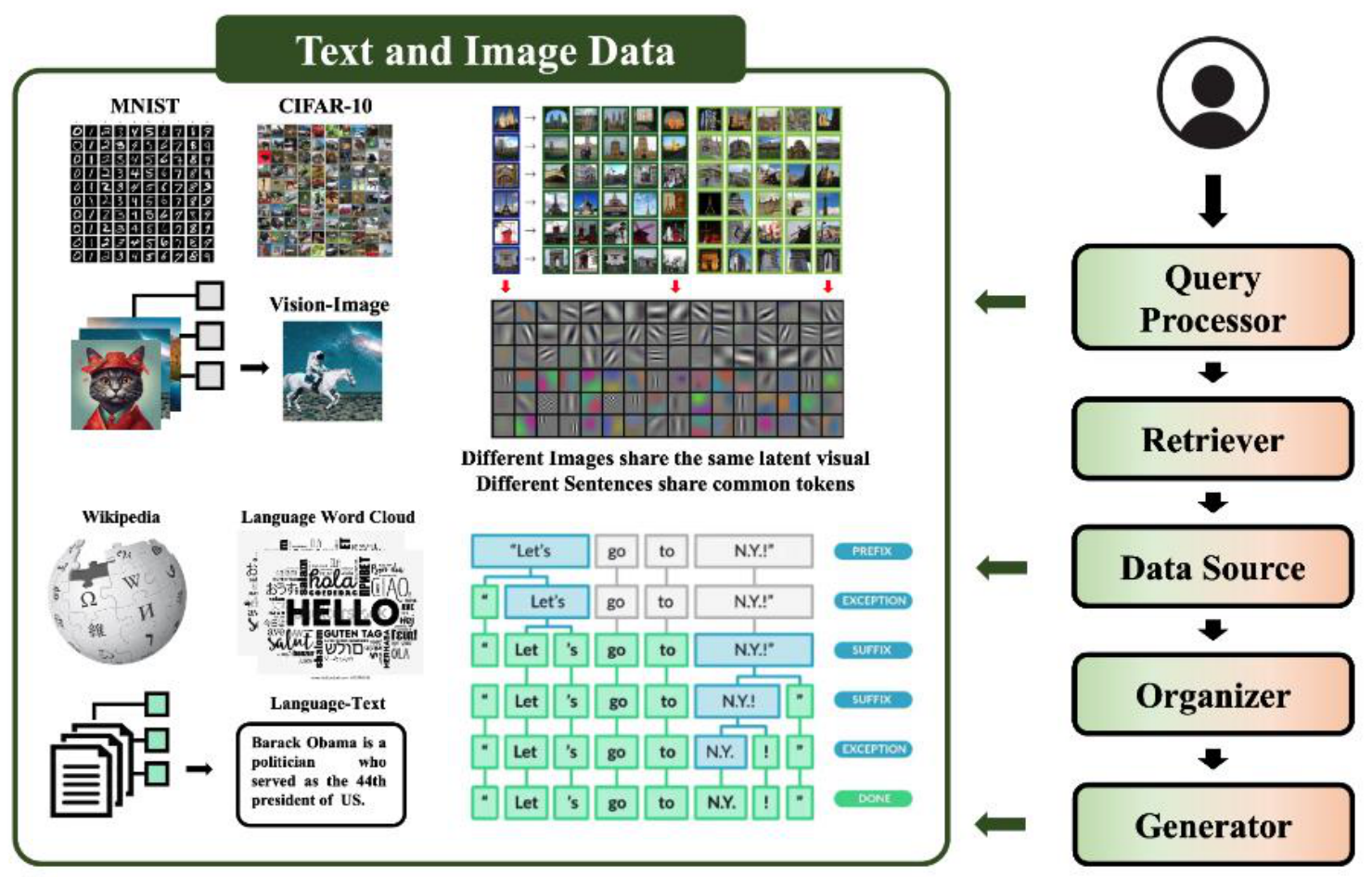
The survey splits every GraphRAG into five parts, and these are the five boxes in the middle of the slide. For our all-deadlines question they look like this: my course example
Part
Job
In our course
Query processor
Make the question searchable
Turn “deadlines” into entities: Proposal, Project milestone, Final report, Homework 1
Retriever
Fetch the useful part of the graph
Walk the due and released edges from these nodes to fetch the dates
Data source
The graph itself
The knowledge graph from step 5
Organizer
Trim and order what was fetched
Write the four relations as four lines of text
Generator
Write the answer
The LLM, which writes the four dates
The left part of the slide shows ordinary RAG data: text and images. According to the survey, text is a line of tokens, and an image is a grid of small patches. Different sentences share the same tokens. Graph data has no shared unit like that, and its structure differs from domain to domain. So each domain needs its own GraphRAG design. from the paper
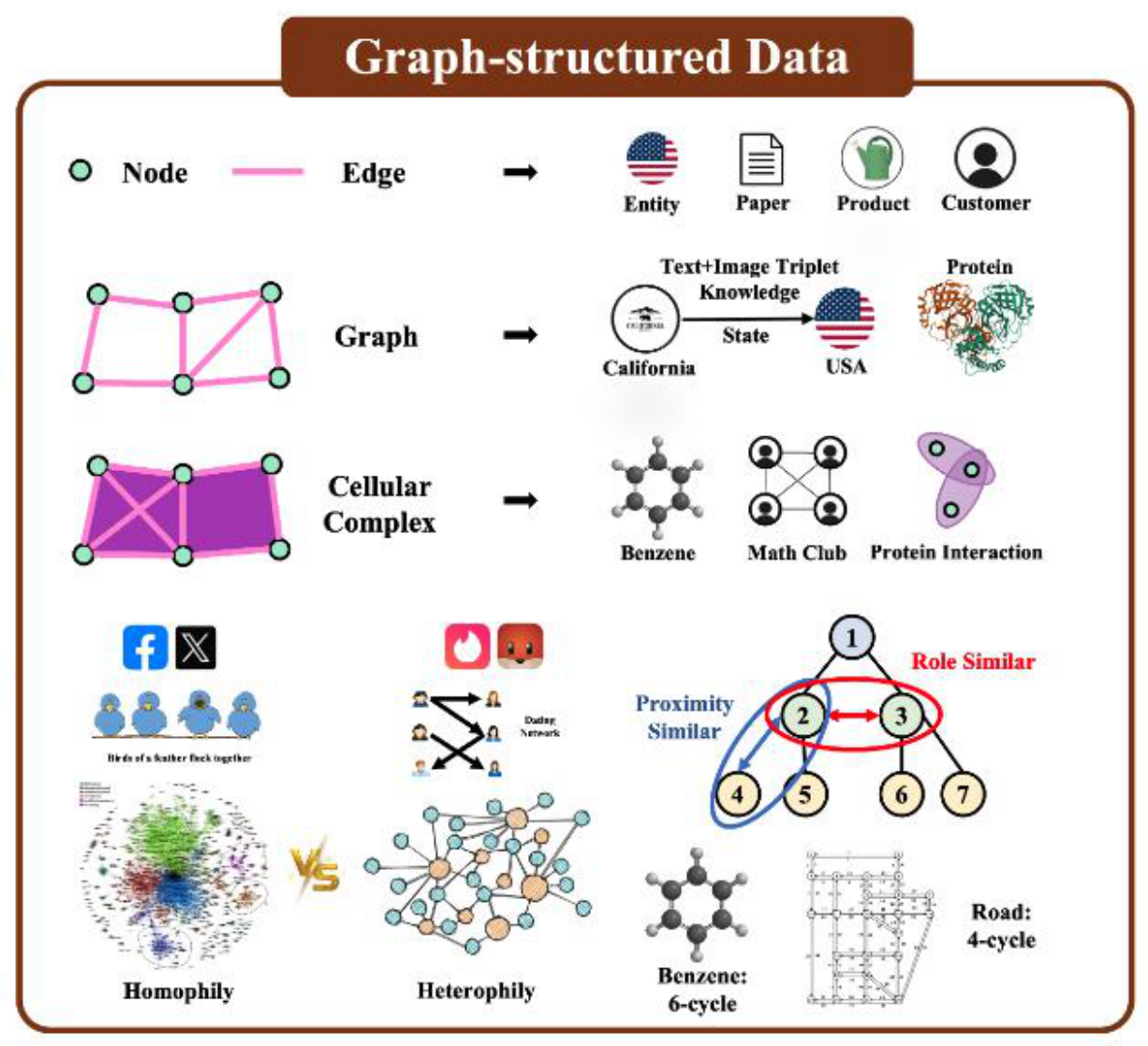
The right part of the slide shows kinds of graphs:
What nodes are: entities, research papers, products or customers. For example, citation edges between papers, or purchase edges between customers and products.
Graph: one row of a knowledge graph, (California, State, USA), which has the same shape as our (Project milestone, due, Week 6). A protein's structure is also a graph.
Cellular complex: besides edges, it has parts that treat several nodes as one unit. Examples are the whole ring of benzene, or the four members of a club who are all linked to each other.
Homophily and heterophily: in homophily, linked nodes are alike, like friends in a social network. In heterophily, linked nodes are of different kinds, as in a dating network.
Proximity similar and role similar: in the slide's tree, 2 and 4 are alike because they are linked. 2 and 3 are not linked, but they hold the same position: both are children of 1, and both have two children. In our graph, Project milestone and Final report are role similar, because both are parts of Project and both have a due date.
6-cycle and 4-cycle: benzene has a ring of 6 nodes, and a street grid has rings of 4 nodes. In drug design or city planning, the retriever has to recognize such shapes.
The survey lists 10 such domains: knowledge, document, scientific, social, planning and reasoning, tabular, infrastructure, biological, scene and random graphs. Edge's GraphRAG belongs to the document graph domain. from the paper
10Now read Stanford's slides yourself
Below are this lesson's four Stanford slides, unchanged. Under each slide are a few questions. Think of the answer first, then open it. If something stops you, go back to the step named in the answer. If a slide looks small on a phone, click the image to open it at full size.
Stanford's RAPTOR slide, and below it its three boxes, enlarged.
Read the RAPTOR slide
In the middle box, which nodes is chunk 5 under, and what kind of clustering is this?
Show the answer
Chunk 5 is in two groups, {3, 5} and {1, 4, 5}, so it sits under both node 6 and node 7. This is soft clustering. In RAPTOR the decision comes from the GMM membership, and in the code a chunk joins a cluster when its membership is above 0.1. (Steps 2 and 6)
The right box shows four things inside node 8. What is the “Text Embedding” [3, .1, 4, .1, 5] used for?
Show the answer
It is the embedding of node 8's summary, and at retrieval time the cosine with the question is computed on this vector. The 5 numbers on the slide are only for illustration. Index #8 is the node's identifier, and Child Nodes 2, 3 say which nodes the summary covers. (Steps 3 and 4)
The last line says a detail question matches a leaf, a thematic question matches a node. Where did you see this, and how does the paper do it?
Show the answer
In the widget of step 4, the milestone question matched the syllabus leaf at 0.99, and the all-deadlines question matched summary A at 1.00. The paper does it with the collapsed tree, which sorts the nodes of all levels in one list. (Steps 4 and 7)
Stanford's Cinderella slide, and below it the tree and the colour legend, enlarged. Orange is the first question's colour, and purple the second's.
Read the Cinderella slide
How many nodes does each level of this tree have? And why are there 4 nodes at the top instead of 1 root?
Show the answer
There are 16 leaves, 0 to 15, then 7 in the middle, 16 to 22, and 4 at the top, 23 to 26. That is 27 nodes in all. RAPTOR stops when further clustering is no longer possible, so several nodes can remain at the top. The tree on the first slide also had two nodes at the top, 9 and 10. (Step 3)
For the first question, the central theme, which levels did RAPTOR choose nodes from?
Show the answer
From all three: 25 from the top, 16, 18 and 19 from the middle, and 11 and 15 from the leaves. For a thematic question most of the nodes are summaries, but two leaves also made it, because RAPTOR matches the question against nodes on every level. (Steps 4 and 7)
For the second question RAPTOR chose only 25, 16, 17 and 19, no leaves. DPR chose the leaves 2, 3, 4, 5 and 11. How does DPR's content reach RAPTOR's context, and what difference did this make to the answer?
Show the answer
Nodes 16 to 26 are summaries of the nodes below them, so the leaves' content reaches them inside the summaries. That is what the slide's last line says. In the paper, GPT-4 given only DPR's context said the happy ending could not be determined. Given RAPTOR's context, it answered correctly. (Steps 4 and 7)
Stanford's GraphRAG slide, and below it the steps and the communities graph, enlarged.
Read the GraphRAG slide
The arrows in the left column say “domain-tailored summarization” twice. Why is extracting entities a kind of summarization, and what does “domain-tailored” mean?
Show the answer
Entities, relations and their descriptions are a short written form of the text, so the paper calls them a kind of summarization. Domain-tailored means the prompt carries examples from the same domain, such as science or law. (Step 8)
Why does “query-focused summarization” appear twice in the right column?
Show the answer
The first time, community summaries become community answers, the map step. The second time, community answers become the global answer, the reduce step. Both times the LLM writes with the question in mind. (Steps 5 and 8)
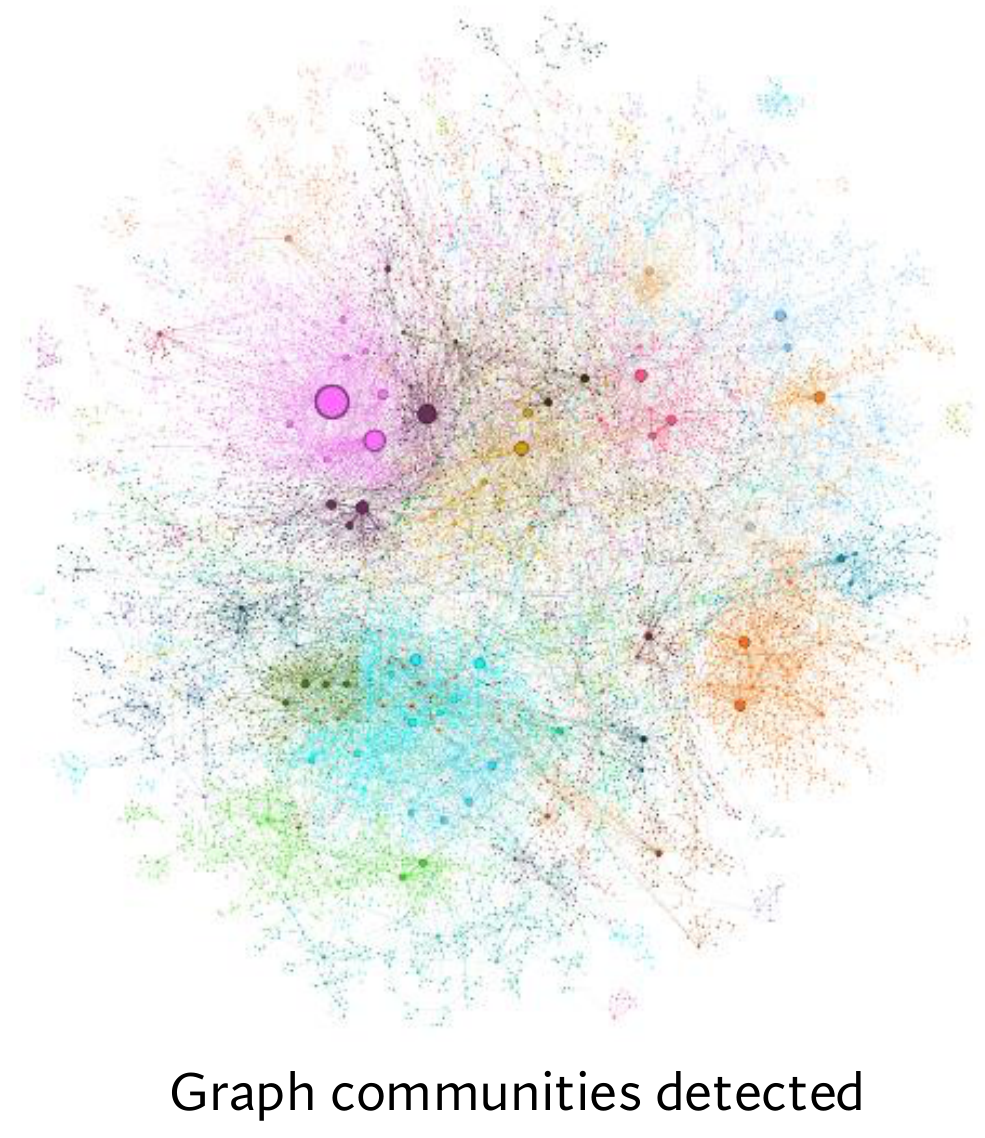
In the picture on the right, what do the colours and the sizes of the circles show?
Show the answer
This is a figure from the paper: Leiden's top-level communities on the graph of the news dataset. Each circle is an entity, its size follows its degree, and its colour shows its community. The big pink circle is an entity with very many edges from the paper. (Step 8)
Stanford's GraphRAG variants slide, and below it its two parts, enlarged.
Read the GraphRAG variants slide
What are the five boxes in the middle, and what would the Retriever do for the all-deadlines question?
Show the answer
Query Processor, Retriever, Data Source, Organizer and Generator. The Retriever would walk the due and released edges from the Proposal, Project milestone, Final report and Homework 1 nodes and fetch all four dates. (Step 9)
In the tree at the bottom right, which node is node 2 proximity similar to, and which is it role similar to?
Show the answer
Proximity similar to node 4, because 2 and 4 are linked by an edge. Role similar to node 3, because both are children of 1 and both have two children, even though they are not linked. (Step 9)
The left part says different sentences share common tokens. Why is nothing like this written for the graphs?
Show the answer
Graph data has no shared unit like a token. A knowledge graph comes in rows, a molecule in rings, and roads in loops, so each domain's GraphRAG is built differently. (Step 9)
3 points from this lesson
A thematic question's answer is not in any single chunk. Every chunk gets a low cosine, raising K is not enough, and a big chunk averages everything away.
RAPTOR uses a GMM to give each chunk a membership for every cluster, and soft clustering lets a chunk sit in more than one cluster. It builds the tree from cluster summaries and searches every level with the collapsed tree. With GPT-4 it reaches 82.6% accuracy on QuALITY, 20.3 points above the previous best.
GraphRAG has an LLM build a knowledge graph, finds levels of communities with Leiden, and writes a global answer with map-reduce. Its comprehensiveness win rate over vector RAG is 72% to 83%, and its top level needs only 2.3% to 2.6% of the tokens of the raw chunks.
New terms in this lesson
Detail question and thematic question
The answer is written in one place, or it is built from several passages. For example, “When is the milestone due?” and “What are all the deadlines?”.
Clustering
Splitting vectors into groups so that the vectors in a group are close to each other. For example, the syllabus [0.1, 0.9] and the project page [0.2, 0.8] have cosine 0.99, so they share a group.
Cluster and centroid
A cluster is a group, and its centroid is the average of its vectors. For example, the centroid of [0.1, 0.9], [0.2, 0.8] and [0.15, 0.85] is [0.15, 0.85].
Soft clustering
Putting one passage into more than one cluster. For example, the FAQ page, whose cosine is high with both centroids (0.86 and 0.78).
RAPTOR
Building a tree bottom up from summaries of clusters, and searching every level. For example, the all-deadlines question matches summary A.
Tree, node, leaf, root
A structure with levels: a node is a box, a leaf is a node at the bottom, and the root is the node at the top. For example, 2 summaries above 6 chunks (the leaves), and 1 root above them.
Entity
Any named thing: a person, a place, a course, a document or a date. For example, Week 6, TAs, Room 104.
Relation
A link between two entities. For example, (Project milestone, due, Week 6).
Knowledge graph and edge
A network of entities (nodes) and relations (edges). For example, an edge labelled “due” between the milestone and Week 6.
Community
A tightly linked part of a graph. For example, Office hours, TAs, Room 104 and Zoom.
GraphRAG
Answering global questions from a knowledge graph, its communities and their summaries. For example, the all-deadlines answer, built from the Project and Homework 1 communities.
Query-focused summarization
Writing a summary with the question in mind. For example, asking for “all the deadlines” makes the Project community's summary give only the dates.
Gaussian mixture model (GMM)
A weighted sum of bell curves: P(x) = ∑ πk 𝒩k(x). It gives every passage a membership for every cluster. For example, [0.6, 0.4] gets 0.904 for office hours and 0.096 for deadlines.
BIC
ln(N) · k − 2 ln(L̂): choosing the number of clusters by weighing the fit's likelihood against its parameter count, where the smallest BIC wins. For example, on 6 passages K = 2 gives −23.64 and K = 3 gives −20.11.
UMAP
Turning vectors into ones with fewer numbers while keeping nearby points nearby. For example, RAPTOR's code makes every vector 10 numbers long.
Tree traversal and collapsed tree
Picking the top k on each level from the top down, or sorting all nodes in one list and taking them up to a token limit. For example, for the all-deadlines question the collapsed tree takes 5 nodes within 100 tokens, A first.
F1
A score that combines precision and recall, 2PR ÷ (P + R). For example, P = 0.75 and R = 0.6 give F1 = 0.667.
Leiden and degree
Leiden splits a graph into communities with many edges inside. A node's degree is its number of edges. For example, Project has degree 3.
Map-reduce
Doing the same job on each piece separately (map), then combining the results (reduce). For example, a partial answer and a score from each community, then a final answer in score order.
Win rate
The percentage of judgments that favour one of two systems, where 50% means a tie. For example, about 450 of 625 judgments, or 72%.