Chunking: cutting documents into pieces for retrieval
Chunking means cutting a long document into small pieces, so that the retriever can make one vector per piece and store it in the index. These pieces are called chunks. The retriever searches for chunks and returns chunks, which is why Stanford's slide calls the chunk the basic unit of retrieval.
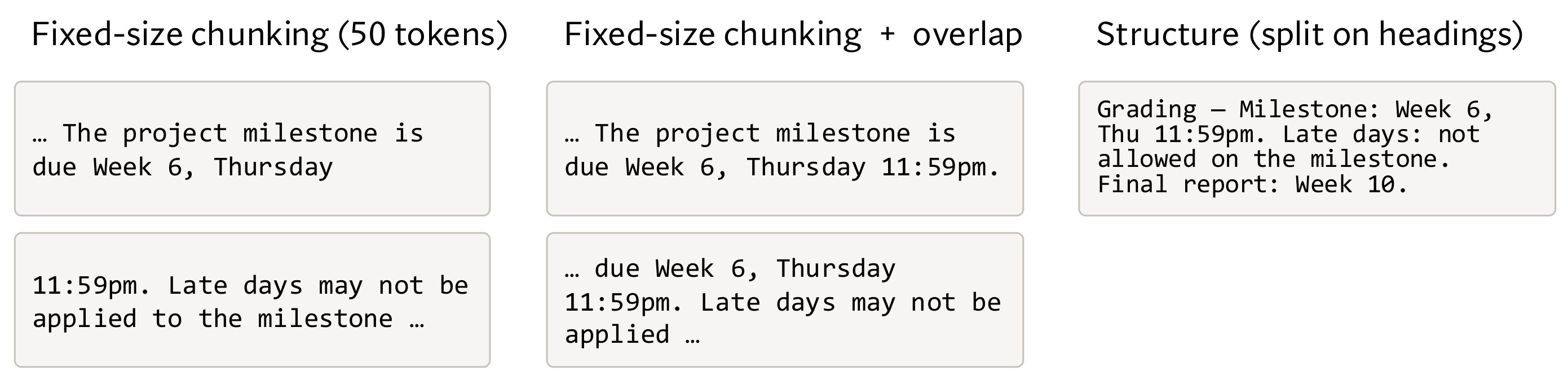
In lesson 2, the answer to when is the project milestone due was in the syllabus passage: Week 6, Thursday 11:59pm. That passage came to us already cut, but the real syllabus is 40 pages long. In the pipeline of lesson 6, cutting it is the first step of building the index. Cut it every 50 tokens, and one chunk ends at …due Week 6, Thursday while 11:59pm. lands in the next chunk. Do not cut it at all, and the milestone's 2 lines dissolve into a single vector for 40 pages.
The ladder for this lesson
The ladder has 8 steps. The first 4 are the same as in the easy version, and steps 5 to 8 take you to the level of the Stanford slides. Under each step you can see what you will be able to do after it.
What you need first: Lesson 1 (token), Lesson 3 (vector, embedding, cosine) and Lesson 6 (indexing time). From step 5 on, Lesson 13 (recall) also helps. If you already know a step, skip to the next one. A word with a dotted underline and ▾ opens its definition when you click it.
1A chunk's vector: the average of its token vectors
Retrieval needs one vector per chunk, and that vector is often the average of the vectors of all the chunk's tokens. The index stores this one vector for each chunk. When a question arrives, the retriever computes the between the question's vector and every chunk's vector, and returns the chunks with the largest cosines. The six passages of lesson 2 were really chunks too.
First, look at where the token vectors come from. An makes a separate vector for every , and the surrounding words affect that vector too. This is called a contextual embedding.
Take the word late, which appears in two sentences: Late days may not be applied and late afternoon office hours. Suppose the first number of a vector stands for office hours and the second for deadlines. A contextual embedding then gives late two different vectors. Older static word embeddings, such as word2vec, kept one vector per word type. A word type is a word as it appears in the dictionary, whatever sentence it is in. my numbers
Sentence
Static: vector for late
Contextual: vector for late
Late days may not be applied
[0.5, 0.5]
[0.1, 0.9]
late afternoon office hours
[0.5, 0.5]
[0.9, 0.1]
Now we need one vector for the whole chunk, which is called a passage embedding. The most common way is to average all the chunk's token vectors: add up the numbers in each column and divide by the number of tokens. This is called mean pooling. Take a small chunk of three tokens: my example
Token
Vector
Office
[0.9, 0.1]
hours
[0.7, 0.3]
Tuesday
[0.8, 0.2]
Mean pooling: the average of each column
[0.8, 0.2]
First column: 0.9 + 0.7 + 0.8 = 2.4, and 2.4 ÷ 3 = 0.8.
Second column: 0.1 + 0.3 + 0.2 = 0.6, and 0.6 ÷ 3 = 0.2.
All three tokens leaned towards office hours, so the chunk's vector [0.8, 0.2] leans the same way. Mean pooling gives every token the same weight, and in step 2 this is exactly what hurts a large chunk.
Think first
Add one more token to the chunk: 4pm, with the vector [0.8, 0.2]. What is the chunk's vector now, and how many numbers does it have?
Show the answer
[0.8, 0.2], and it still has 2 numbers. First column: (0.9 + 0.7 + 0.8 + 0.8) ÷ 4 = 3.2 ÷ 4 = 0.8. Second: (0.1 + 0.3 + 0.2 + 0.2) ÷ 4 = 0.8 ÷ 4 = 0.2. Whether a chunk has 3 tokens or 300, the average has as many numbers as each token vector. So every chunk's vector has the same count of numbers, and the index can compare them all.
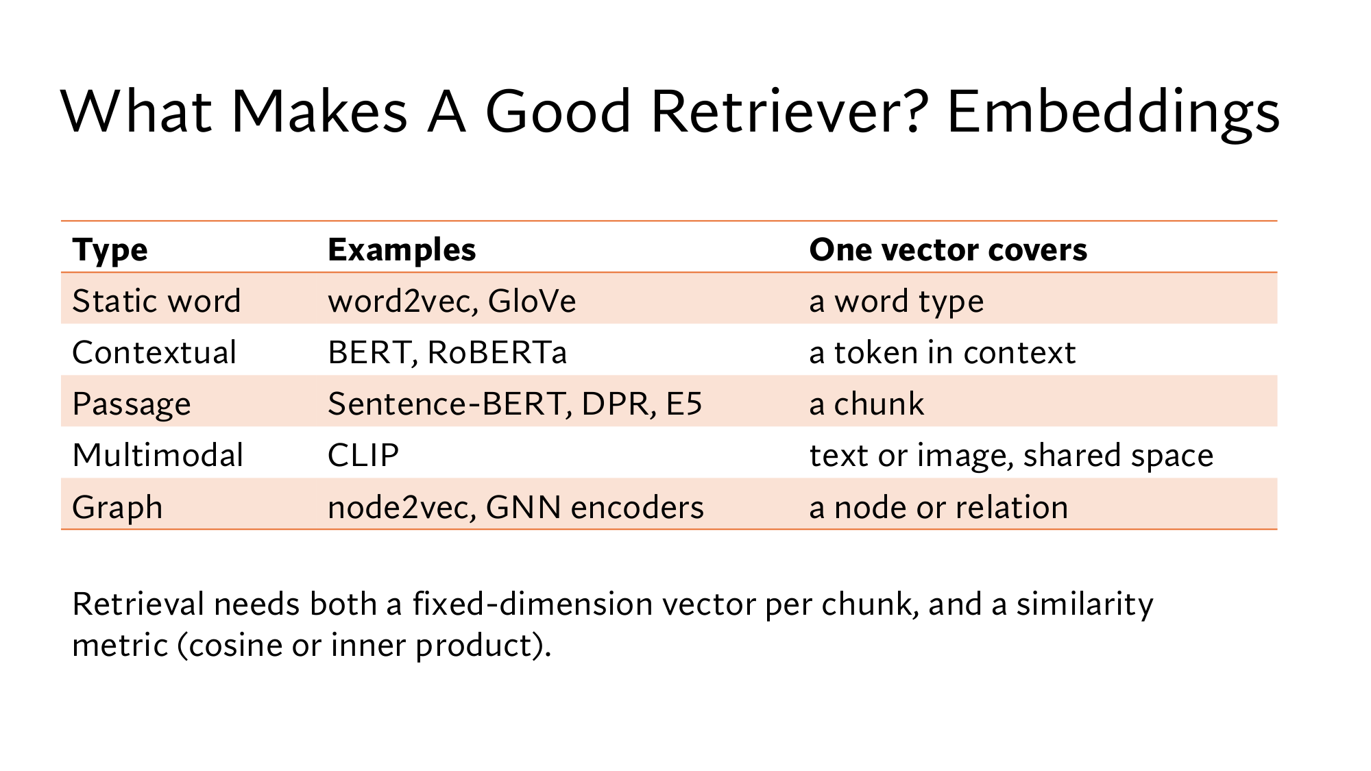
Stanford's embeddings slide makes the same point. Its table lists five kinds of embeddings, and you have just met the top three: static word, contextual and passage. The other two, and , are vectors for images and for networks. The slide's last line names two things retrieval needs. The first is one vector per chunk, with a fixed . The second is a way to compare vectors, cosine or inner product.
Stanford's slide: What Makes A Good Retriever? Embeddings. In the passage row, one vector covers one chunk, and this lesson is about that chunk. Click the image to open it at full size.
2Chunk size: small loses context, large gets averaged away
A large chunk becomes the average of many topics, and a small chunk loses its context. So choosing a chunk size means choosing between two opposite problems, and Stanford's slide lists both.
A large chunk: topics get averaged together
Suppose the office hours topic has the vector [1, 0] and the deadline topic has [0, 1]. If a large chunk holds both topics in equal parts, mean pooling gives [0.5, 0.5]. The query office hours has the vector [1, 0]. my example
The cosine from lesson 3 is the dot product of two vectors divided by the product of their . A small chunk about office hours only, [1, 0], has cosine 1 with the query, because the two point in the same direction. The large chunk's cosine takes three steps:
Dot product: 1 × 0.5 + 0 × 0.5 = 0.5.
Lengths: the query's length is 1, and the length of [0.5, 0.5] is √(0.5² + 0.5²) = √0.5 = 0.707. The square root √ is the number that gives the number inside when multiplied by itself. Check: 0.707 × 0.707 = 0.5.
Cosine: 0.5 ÷ (1 × 0.707) = 0.71.
Chunk
Vector
Cosine with the query
Small chunk, office hours only
[1, 0]
1.00
Large chunk, office hours and deadlines
[0.5, 0.5]
0.71
The large chunk does contain the right fact, yet its cosine fell from 1.00 to 0.71, because the deadline topic was mixed into the average. Any other chunk with a cosine of 0.8 now ranks above it. The 40-page syllabus covers office hours, deadlines, grading and the project, so there the cosine falls even further.
Think first
A chunk holds three topics in equal parts: [1, 0, 0], [0, 1, 0] and [0, 0, 1]. What vector does mean pooling give, and what is its cosine with the query [1, 0, 0]?
Show the answer
The average is [1/3, 1/3, 1/3], and its dot product with the query is 1/3. Its length is √(3 × 1/9) = √(1/3) = 0.577. Cosine = (1/3) ÷ (1 × 0.577) = 0.58. Two topics gave 0.71 and three give 0.58, so the more topics, the lower the cosine.
A small chunk: the context is left behind
Now go the other way and make very small chunks. The queue log has 19 words, and cutting it into chunks of 5 words gives these 4 chunks:
Chunk 1 · 5 words
Queue log, last 3 weeks:
Chunk 2 · 5 words
Tuesday 4pm office hour averaged
Chunk 3 · 5 words
14 students waiting; Thursday 9am
Chunk 4 · 4 words
office hour averaged 3.
The fourth chunk has the 3, but it does not say which day's office hour that is. Thursday 9am went into the third chunk, so the fourth chunk's vector does not know it either. The answer to lesson 2's question, which office hour is least crowded, is no longer complete in any single chunk.
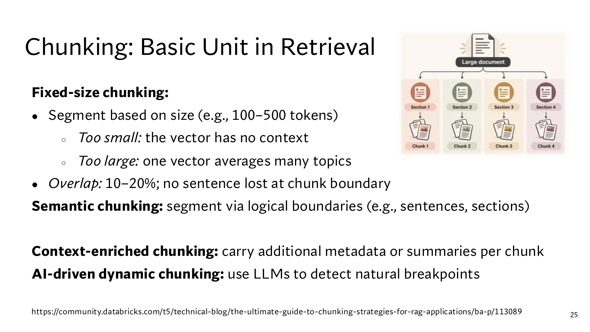
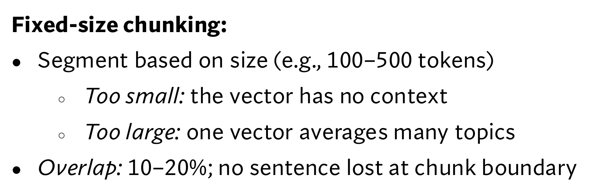
Fixed-size chunking takes the middle road: every chunk gets a fixed number of tokens. Stanford's slide gives 100 to 500 tokens as an example.
Small chunks are good for precise questions, but they lose their context. Large chunks get more context, but their one vector becomes the average of many topics. Lesson 8 gives a small chunk its lost context back, and lesson 9 builds a layer of summaries above the chunks for broad questions.
3Overlap and stride: saving a fact cut at a boundary
With overlap, every new chunk starts by repeating the last few tokens of the previous chunk, so that a fact cut at a boundary survives whole. You need it because whatever size you choose, some fact will fall on a boundary. That is exactly how the milestone date was cut at 50 tokens. Stanford's slide recommends an overlap of 10 to 20%.
The distance between the starts of two neighbouring chunks is called the stride: stride = chunk size − overlap. With chunk size 9 and overlap 6 the stride is 3, so chunks start at words 0, 3, 6, 9, ….
Now cut the beginning of the syllabus in the widget below. Treat every word as one token, and count from 0. The milestone fact, milestone is due Week 6, Thursday 11:59pm., is 7 words long and sits at words 3 to 9 of the syllabus. With chunk size 9 and overlap 0, the first chunk covers words 0 to 8, so 11:59pm. falls outside it.
Think first
Keep the chunk size at 9 and raise the overlap from 0 to 6. At what overlap does the date first appear whole in a single chunk? Guess first, then check in the widget.
Show the answer
Only at overlap 6. The stride is then 3, and the second chunk runs from word 3 to word 11, which holds the whole date. With overlap 1 to 5, no chunk starts at word 3 or earlier and still reaches word 9.
Cut the syllabus into chunks
The underlined fact, the milestone date, should be whole inside one chunk. Words with a light background are overlap.
How much overlap is enough
You can count out why it has to be 6. A chunk of 9 words holds the fact at words 3 to 9 only if it starts at word 1, 2 or 3. Chunks start at 0, stride, 2 × stride, …, and a start is certain to land on one of those 3 positions only if the stride is 3 or less. With stride 4 the starts are 0, 4, 8, which miss 1, 2 and 3 altogether. The stride is 9 − overlap, so the overlap must be at least 6.
The same count works for any size. With chunk size C and a fact of L words, there are C − L + 1 good starting positions for a chunk. Here that was 9 − 7 + 1 = 3. If the stride, which is C − overlap, is no larger than that, you get this rule: this rule is not on the slide, it follows from counting
overlap ≥ L − 1, and chunk size ≥ L
Here L = 7, so the overlap must be at least 6. If the chunk is shorter than the fact, no overlap can bring the fact into one chunk.
Think first
Set the widget to chunk size 10 and overlap 0. The date shows up whole. Is that a reliable defence?
Show the answer
No, that is luck. The first chunk covers words 0 to 9, and the date ends exactly at word 9. With one more word at the start of the syllabus, 11:59pm. would sit at word 10 and fall into the next chunk. An overlap of L − 1 protects the fact wherever it sits.
What overlap costs
Overlap is not free, because the repeated tokens go into two chunks. Cut a document of 1,000 tokens into chunks of 50 tokens, and without overlap you get 1,000 ÷ 50 = 20 chunks. With an overlap of 10 tokens, which is 20%, the stride is 40. Chunks then start at tokens 0, 40, …, 960, because the chunk starting at 960 already reaches the end of the document. That makes 960 ÷ 40 + 1 = 25 chunks.
So 20% overlap means 25% more embeddings to compute and store in the index.
4Cutting by meaning: headings, metadata and LLMs
Semantic chunking cuts the text where the text already divides itself, such as at the end of a sentence or a section. You need it because fixed-size chunking cuts by count and ignores the text's structure. Set the widget to chunk size 20 and overlap 0. The second chunk starts with final report is due Week 10. and runs on into the office hours part, so one chunk holds two topics.
Each part of the syllabus has its own heading: Grading, Office hours and Project. Splitting on headings is the simplest form of semantic chunking. Press Split on headings in the widget. The syllabus splits into 3 chunks of 26, 16 and 12 words, and each chunk is about one topic. The chunks are no longer the same size, and that is the price of this method.
A small chunk can still lose its context. Late days may not be applied to the milestone. does not say on its own which course it belongs to. Context-enriched chunking handles this by storing extra information with every chunk, such as metadata or a short summary.
Metadata is data about data: the document's name, the section and the date. A context-enriched chunk could look like this: my example
[Source: CS 329Z syllabus, section: Grading, updated: 30 Sep 2026] Late days may not be applied to the milestone.
Now even the small chunk says which course and which section it comes from. Lesson 8 shows the most effective form of this idea, where an LLM writes context for every chunk.
The last method is AI-driven dynamic chunking. It asks an LLM where the topic changes in the text, and cuts there. It works even without headings. But every document has to pass through the LLM once, which costs time and money.
Method
Benefit
Cost
Fixed-size
Simple, every chunk the same size
A fact can break in the middle
Fixed-size + overlap
A broken fact is whole in the next chunk
More chunks, repeated text
Semantic, such as headings
Each chunk is about one topic
Chunk sizes vary
Context-enriched
Even a small chunk carries its context
Metadata or summaries must be made
AI-driven
Meaningful boundaries even without headings
LLM calls for every document, slow and expensive
Now go back to the opening problem. Splitting on headings puts the whole milestone date into the Grading chunk, and that chunk is about a single topic. So the broken date and the averaged-away vector are both solved at once for this document. Not every document has clean headings, which is why the other methods are useful too.
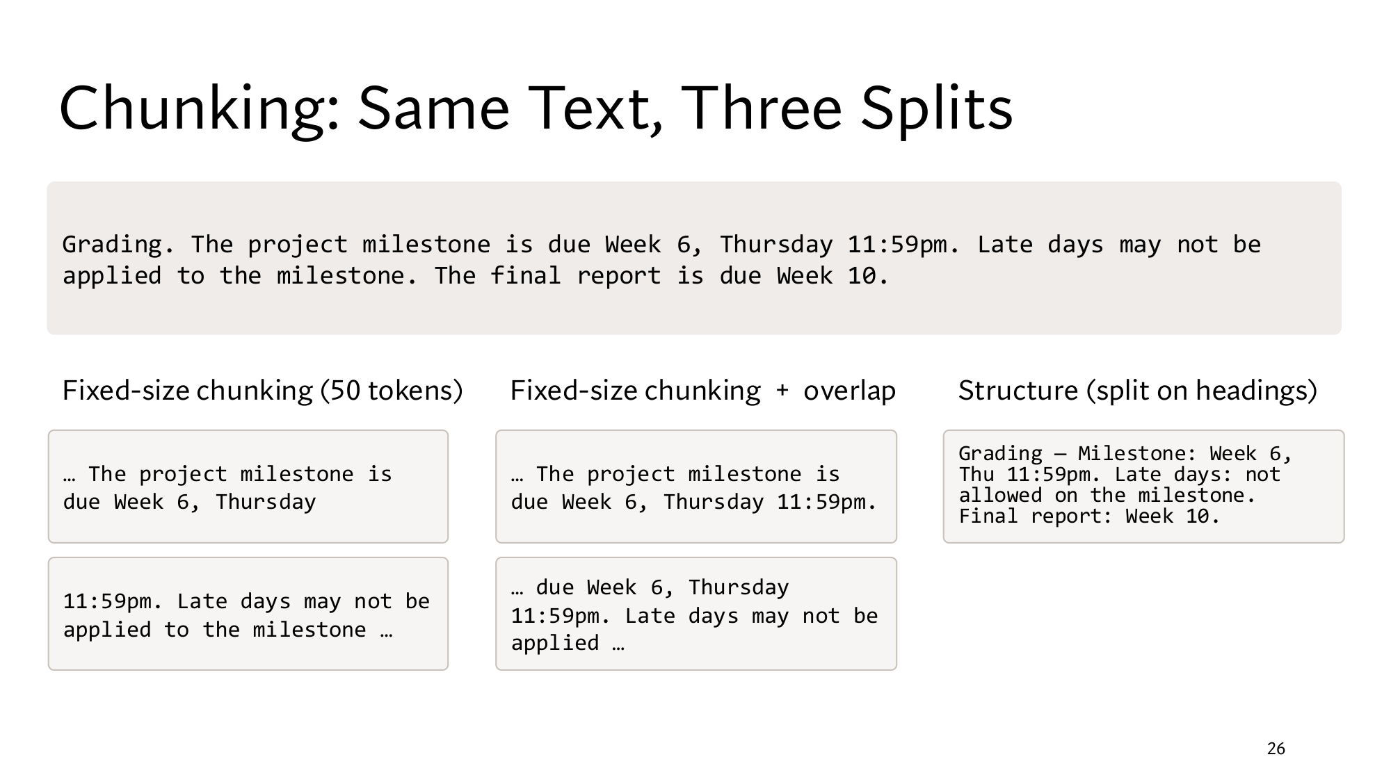
You can now read both of Stanford's chunking slides. The first lists all four methods, and the second cuts our syllabus in three ways.
Stanford's slide: Chunking: Basic Unit in Retrieval. At the top are fixed-size chunking and overlap (steps 2 and 3), and below them the other three methods (step 4).Stanford's slide: Chunking: Same Text, Three Splits. Our syllabus is at the top. Below it, on the left, is the date broken at 50 tokens, in the middle the date saved by overlap, and on the right a chunk split on headings and rewritten more tidily.
From here: the Stanford level
The 4 steps above are the same as in the easy version. The 4 steps below take you to the level of the Stanford slides: the full maths of mean pooling and overlap, then the inside story of the methods from the slide's source, the Databricks guide, and finally reading the slides yourself. Every piece of maths is explained where it first appears.
5The maths of mean pooling: how much a fact gets diluted
Mean pooling gives every token a weight of 1/N, so a fact affects the chunk's vector only as much as its share of the chunk. Step 2 showed this for two topics. This step runs the same arithmetic for any number of topics and any share.
First, write mean pooling in symbols. The chunk has N tokens, and token t has the vector ht. Take the of all the vectors and divide by N:
hchunk = 1N ∑t=1N ht
In step 1, N = 3, with h1 = [0.9, 0.1], h2 = [0.7, 0.3] and h3 = [0.8, 0.2], and the result was [0.8, 0.2]. Adding and dividing do not change how many numbers there are, so hchunk has as many numbers as each ht. BERT-base gives every token a vector of 768 numbers, so a chunk of 100 tokens and a chunk of 500 tokens both get a vector of 768 numbers.
Not every model takes the average. According to lesson 3, DPR uses the vector of a special token called [CLS] for the whole passage, while Sentence-BERT uses mean pooling. Both keep the vector's dimension fixed, which is the condition on the slide's last line.
k equal topics: cosine 1/√k
Now take a toy model in which every token's vector points exactly in its topic's direction, and the directions of different topics are at 90° to each other, so their cosine is 0 my model. Suppose a chunk holds 4 topics in equal shares. Each topic's share is then 1/4, and mean pooling gives [0.25, 0.25, 0.25, 0.25]. The query for the first topic is [1, 0, 0, 0].
Dot product: 1 × 0.25 = 0.25, because the query's other numbers are 0.
With k topics the same steps go like this. Every number is 1/k, so the dot product is 1/k. The length is √(k × 1/k²) = √(1/k) = 1/√k. The cosine is (1/k) ÷ (1/√k), and since k = √k × √k this becomes 1/√k:
cosine = 1√k
Equal topics in the chunk, k
Cosine with the query, 1/√k
1
1.00
2, the large chunk from step 2
0.71
3, the question in step 2
0.58
4
0.50
10
0.32
100
0.10
In the table the cosine falls fast at first, then slowly. Multiplying k by 4 doubles √k, so the cosine halves: 1.00 at k = 1, and 0.50 at k = 4.
Think first
At k = 4 the cosine is 0.50. What is it at k = 25, and at 100?
Show the answer
At k = 25 it is 1/√25 = 1/5 = 0.20, and at k = 100 it is 1/10 = 0.10. From 25 to 100, k grew 4 times, and the cosine halved from 0.20 to 0.10.
A fact with a small share almost disappears
Real chunks do not hold topics in equal shares. Suppose a share f of the chunk is about office hours and the remaining 1 − f is about deadlines. Mean pooling then gives [f, 1 − f], and the cosine with the query [1, 0] is:
cosine = f√(f² + (1 − f)²)
Look at f = 0.2. The vector is [0.2, 0.8], and its dot product with the query is 0.2. Its length is √(0.04 + 0.64) = √0.68 = 0.825, so the cosine is 0.2 ÷ 0.825 = 0.24.
Share of office hours, f
Cosine with the query
1
1.00
0.9
0.99
0.5
0.71
0.2
0.24
0.1
0.11
0.01
0.01
When f is small, 1 − f is close to 1, and so is the square root underneath. The cosine is then roughly f itself. So a fact that makes up 1% of a chunk gets a cosine of about 0.01.
Now go back to the 40-page syllabus from the opening. Suppose each page has 50 lines, 2,000 lines in all, and the milestone fact takes 2 lines my numbers. Then f = 2 ÷ 2,000 = 0.001, and in this toy model the query's cosine with a single vector for the whole syllabus is also about 0.001. Real encoder vectors are not this clean, but mean pooling always gives a small share a small weight.
Watch out: The Databricks guide that the slide cites names one more limit. Embedding models and LLMs both have a strict limit on input size, and well-sized chunks stay within it from the Databricks guide. So putting 40 pages into one vector is often not even possible.
6The full arithmetic of overlap: the chance a fact survives, and the chunk count
Even when the overlap is below L − 1, a fact sometimes survives whole, and the chance of that is (C − L + 1) ÷ stride. The rule in step 3 was about a guaranteed defence. This step shows how much risk a smaller overlap carries, and what overlap costs.
The chance a fact survives too little overlap
In step 3 you saw that a chunk has C − L + 1 good starting positions. Chunks start every stride words. Now suppose the fact can start anywhere in the document, with every position equally likely my model. Then out of any stride consecutive positions, the fact lands whole in some chunk for C − L + 1 of them.
With size 9 and overlap 0 the stride is 9, and the good positions number 9 − 7 + 1 = 3. So the fact survives at 3 positions out of 9, which is 3 ÷ 9 = 33.3%, and it is cut 66.7% of the time. The syllabus date in step 3 fell into that 66.7%. With size 10 and overlap 0 the chance is (10 − 7 + 1) ÷ 10 = 40%, so the luck in step 3 was a 40% chance.
chance = min(1, C − L + 1C − overlap)
min(1, x) means the smaller of 1 and x, because a chance cannot exceed 1. If the stride, the C − overlap at the bottom, is at most C − L + 1, the chance is 1. That is exactly the rule from step 3, overlap ≥ L − 1.
Chunk size C, overlap
Stride
7-word fact survives
9, 0
9
3/9 = 33.3%
10, 0
10
4/10 = 40%
9, 5
4
3/4 = 75%
9, 6
3
100%
50, 0the slide's 50-token chunk
50
44/50 = 88%
50, 510% overlap
45
44/45 = 97.8%
50, 1020% overlap
40
100%
With 50-token chunks and no overlap, a 7-token fact is cut 12% of the time, which is (L − 1) ÷ C = 6 ÷ 50. With 10% overlap this drops to 2.2%, and with 20% to 0.
When the slide's 10 to 20% advice is enough
The slide says that with 10 to 20% overlap no sentence is lost at a chunk boundary. In tokens the overlap is r × C, where r is the overlap share, such as 0.2 for 20%. By the rule from step 3, this guarantees sentences of up to overlap + 1 tokens:
Chunk size
10% overlap protects
20% overlap protects
100 tokens
up to 11 tokensoverlap 10
up to 21 tokensoverlap 20
200 tokens
up to 21 tokensoverlap 20
up to 41 tokensoverlap 40
500 tokens
up to 51 tokensoverlap 50
up to 101 tokensoverlap 100
So the slide's claim holds for large chunks, but with 100-token chunks and 10% overlap a 30-token sentence can be cut. The claim depends on the chunk size and on how long the sentences are.
Think first
Most sentences in your documents are shorter than 30 tokens, and the chunk size is 200 tokens. What is the smallest overlap that keeps every such sentence whole? What percentage of the chunk size is that?
Show the answer
L = 30, so the overlap must be at least 29 tokens. 29 ÷ 200 = 14.5%, which is inside the slide's 10 to 20% range.
A formula for the chunk count, and the cost of overlap
In step 3, 1,000 tokens with chunk size 50 and stride 40 gave 25 chunks. The last chunk starts where 50 tokens reach the end of the document, which is at token 950 or later. Among 40, 80, 120, … the first such number is 960, and from 0 to 960 there are 960 ÷ 40 + 1 = 25 starts. The same count fits in one formula, where N is the number of tokens in the document:
chunks = ⌈N − Cstride⌉ + 1
⌈x⌉ means the smallest whole number that is x or larger, such as ⌈23.75⌉ = 24 and ⌈19⌉ = 19. Check: (1,000 − 50) ÷ 40 = 23.75, so 24 + 1 = 25 chunks. Without overlap, (1,000 − 50) ÷ 50 = 19, so 19 + 1 = 20 chunks. The formula is for documents longer than one chunk.
For a long document the chunk count is close to N ÷ stride. So overlap multiplies the number of embeddings by about C ÷ stride. If the overlap share is r, the stride is C × (1 − r), and that factor becomes 1 ÷ (1 − r):
Overlap share, r
Times as many embeddings, 1 ÷ (1 − r)
0
1.00
10%
1.11
20%
1.25
25%
1.33
50%
2.00
75%
4.00
This fraction grows slowly at first and then fast, because the 1 − r at the bottom heads towards 0. The slide's 10 to 20% sits in the cheap part: 11% to 25% more embeddings.
Now run it on the 40-page syllabus. Suppose each page holds 500 tokens, so N = 20,000 my estimate. At the two ends of the slide's 100 to 500 token range, the counts are:
Chunk size, overlap
Stride
Chunks
100, 0
100
200
100, 20 (20%)
80
250⌈19,900 ÷ 80⌉ + 1 = 249 + 1
500, 0
500
40
500, 100 (20%)
400
50⌈19,500 ÷ 400⌉ + 1 = 49 + 1
Overlap has one more cost. The overlapping tokens sit in two neighbouring chunks, so the same fact can appear twice in the top K and use up space in the prompt.
7The methods from the inside: the Databricks guide
The chunking slide cites a Databricks guide for its methods, and the guide explains each method with code. The guide is a 2025 technical blog on the Databricks community site: The Ultimate Guide to Chunking Strategies for RAG Applications with Databricks. The 10 to 20% advice comes from it as well. This step runs the guide's inside details on our syllabus. Points that are in the guide but not on the slide are marked from the Databricks guide.
Size and overlap by kind of content
The slide only gives 100 to 500 tokens as an example. The guide splits that up by kind of content: from the Databricks guide
Content
Chunk size
Overlap
General text
200 to 500 tokens
10 to 20%
Code or very technical text
100 to 200 tokens
15 to 25%
Narrative text
500 to 1,000 tokens
Not in the listthe code uses 100 on 800, which is 12.5%
The guide also says to start by running fixed-size chunking at several sizes, such as 100, 200, 500 and 1,000, and to measure the results. For measuring, it names context precision and context recall: how little unneeded text the chunks carry, and how completely they capture everything a question needs. It mentions a MongoDB study in which chunks of about 100 tokens with about 15 tokens of overlap worked best for Python documentation from the Databricks guide. How to measure recall is the subject of lesson 13.
Watch out: The guide's advice is in tokens, but its code counts chunk_size in characters, because it uses Python's len from the Databricks guide. Check first whether your own splitter counts tokens, words or characters.
Recursive splitting: from large separators to small ones
Recursive chunking cuts along a ladder of separators. It cuts at the largest separator first, and any piece that is still larger than the chunk size gets cut at the next smaller separator. In the guide's code the ladder is: a blank line, meaning a paragraph, then a new line, then . at the end of a sentence, then a space, and finally any character from the Databricks guide. For code, the guide suggests separators such as def and class.
Set the chunk size to 20 words on our syllabus, and suppose every section ends with a blank line my example. The first cuts then fall on the blank lines, which gives three sections. Office hours has 16 words and Project has 12, so each becomes one chunk. Grading has 26 words, more than 20, so it is cut into sentences:
Sentences: Grading. (1 word), the milestone sentence (9), the late days sentence (9), and the final report sentence (7).
Join them in order until 20 would be passed: 1 + 9 + 9 = 19. Adding the next sentence would make 26, so the first chunk stops at 19 words.
The second chunk is the final report sentence, 7 words long.
The milestone date is whole, and no sentence is cut in the middle. In the widget, fixed size 20 ended the first chunk at The and pushed final report into the next chunk. The guide's semantic chunking example is in fact this same recursive splitter. from the Databricks guide
Finding boundaries with sentence vectors
Even without headings you can find where the topic changes. The guide says that consecutive pieces that are highly similar can be merged into one chunk from the Databricks guide. The method goes like this: make a vector for every sentence, compute the cosine of each pair of neighbouring sentences, and cut where the cosine drops sharply. Take these vectors for four sentences of the syllabus: my numbers
Sentence
Vector
Cosine with the next sentence
The project milestone is due…
[0.1, 0.9]
0.99
Late days may not be applied…
[0.2, 0.8]
0.99
The final report is due Week 10.
[0.1, 0.9]
0.22
Tuesday 4pm in Room 104…
[0.9, 0.1]
–
Dot product of the final report sentence and the Tuesday sentence: 0.1 × 0.9 + 0.9 × 0.1 = 0.18.
The first two cosines are 0.99. For milestone and late days, for example, it is 0.74 ÷ (0.906 × 0.825) = 0.74 ÷ 0.747 = 0.99. With a threshold such as 0.5, the only cut falls between the third and fourth sentences, exactly at the Office hours heading. Without any headings we got the same split. The cost is one encoder call per sentence, and you have to pick the threshold yourself, because the guide gives none.
Metadata, summaries and filters
In the guide's context-enriched example, every chunk gets a summary of its neighbouring chunks, one on each side. An LLM writes this summary, from a prompt that starts Provide a brief summary of the following textfrom the Databricks guide. According to the guide, metadata such as the section title, the document type and the date also helps with filtering.
On our corpus such a filter is easy to see. If every chunk's metadata holds a date, the retriever can drop chunks older than 2025 before ranking. The old 2024 forum post then never reaches the ranking at all. The guide also names the cost: storage and memory grow, and without care the same information repeats across many chunks from the Databricks guide. Lesson 8 shows the most effective form of this idea, and lesson 18 uses metadata dates to catch stale and conflicting sources.
The cost of chunking with an LLM
In the guide's AI-driven example, the whole document goes to the LLM in one prompt, along with a few instructions. Each chunk should hold a complete idea, complex sections should get smaller chunks, a heading should stay with its content, the order should not change, and there should be no more than a set number of chunks. The LLM answers with a JSON list of the chunk texts. from the Databricks guide
This means the LLM reads the whole document and then writes the whole document again. For the 20,000-token syllabus that is about 20,000 input tokens and 20,000 output tokens, 40,000 tokens of work, while fixed-size chunking needs no LLM at all. The guide's code caps the answer at max_tokens = 4000, so a document longer than about 4,000 tokens cannot come back whole in one call from the Databricks guide. The guide's own list of drawbacks agrees: the result depends on the LLM, compute and API calls are expensive, and getting the same chunks every time is hard.
The guide lists two more methods that are not on the slide. Adaptive chunking gives complex parts smaller chunks and simple parts larger ones. Hierarchical chunking keeps several levels, such as section, subsection and paragraph from the Databricks guide. RAPTOR in lesson 9 builds levels of summaries above the chunks.
Think first
You have a company HR policy. It has clear headings, and each section is 150 to 400 tokens long. Which method would you use, and why?
Show the answer
Splitting on headings, that is, semantic chunking. Each section is already about one topic, and its size is close to the guide's 200 to 500 tokens for general text. Also store the section title and the date as metadata, so that even a small chunk carries its context and an outdated policy can be filtered out. LLM chunking is not needed here, because the boundaries are already clear.
8Now read Stanford's slides yourself
Below are this lesson's three Stanford slides, unchanged. Under each slide are a few questions. Think of the answer first, then open it. If something stops you, go back to the step named in the answer. If a slide looks small on a phone, click the image to open it at full size.
Stanford's embeddings slide, and below it the last line, enlarged. Read each row of the table in the dense version of lesson 3. The questions here are about the chunk part.
Read the embeddings slide
The last line asks for a fixed-dimension vector per chunk. The Grading chunk from the heading split has 26 words, and the Project chunk has 12. After mean pooling, how many numbers does each vector have?
Show the answer
The same as each token vector: 2 in our toy, and 768 in BERT-base. Averaging N vectors does not change the count of numbers, it only divides by N. (Steps 1 and 5)
The passage row says one vector covers one chunk. How many vectors does our syllabus put into the index when split on headings, and how many with fixed-size chunks of size 9 and overlap 6?
Show the answer
3 vectors when split on headings, and 16 with size 9 and overlap 6, because stride 3 over 54 words makes 16 chunks. The widget shows both counts. (Steps 3 and 4)
Stanford's slide: Chunking: Basic Unit in Retrieval. The picture at the top right splits a large document into sections, and each section into chunks. Below are the fixed-size part and the other three methods, enlarged.
Read the chunking slide
Too large: one vector averages many topics. What is the cosine between a chunk with 10 equal topics and a query about one of them?
Show the answer
1/√10 = 0.32. A chunk with one topic would give 1.00. In the toy model of step 5, the more topics, the lower the cosine. (Steps 2 and 5)
The overlap line says that with 10 to 20% overlap no sentence is lost at a boundary. With 100-token chunks and 10% overlap, does a 30-token sentence survive?
Show the answer
Not for certain. 10% overlap is 10 tokens, which protects sentences of up to 11 tokens. A 30-token sentence needs an overlap of 29, which is 29%. In the model of step 6, with stride 90, such a sentence survives (100 − 30 + 1) ÷ 90 = 78.9% of the time and is cut 21.1% of the time. (Steps 3 and 6)
Both context-enriched and AI-driven chunking can use an LLM. How does the LLM's job differ between them?
Show the answer
In context-enriched chunking the boundaries stay as they were, and the LLM writes a summary that is attached to each chunk. In AI-driven chunking the LLM decides the boundaries itself, and in the guide's example it writes the whole document out again as chunks. (Steps 4 and 7)
Stanford's slide: Chunking: Same Text, Three Splits. Below it, the syllabus text and the three methods, enlarged.
Read the three-splits slide
In the middle column, which words appear in both chunks? Which chunk holds the whole milestone fact, and would this overlap always be enough?
Show the answer
On the slide, due Week 6, Thursday 11:59pm. appears in both chunks, so at least 5 words. More words may be hidden behind the “…”. The whole fact, milestone is due Week 6, Thursday 11:59pm., is in the first chunk. To protect a 7-word fact wherever it sits, the overlap must be at least 6. So the slide shows one case in which the fact survived, not a guarantee. (Steps 3 and 6)
How is the chunk in the right-hand column different from the other two?
Show the answer
It is split at the Grading heading, so it holds the whole section and a single topic. Someone has also tidied and rewritten its text: Thu instead of Thursday, and Late days: not allowed on the milestone. So it combines splitting on headings with rewriting the chunk. (Steps 4 and 7)
The text at the top of the slide has 26 words. How would the widget's fixed size 20 cut it, and how would splitting on headings cut it?
Show the answer
With size 20 the first chunk covers words 0 to 19 and ends at The. The second chunk is final report is due Week 10. The date survives, but the final report sentence is broken. Split on headings, the whole text is a single chunk, because it is the entire Grading section. (Steps 3 and 4)
3 points from this lesson
Retrieval needs one vector per chunk, and it is often the average of the contextual token vectors, which is mean pooling. However many tokens there are, the vector keeps the same dimension.
In mean pooling a fact counts only as much as its share. With k equal topics the cosine is 1/√k, and a fact that makes up 1% of a chunk gets a cosine of about 0.01.
With an overlap of L − 1 a fact of L tokens is certain to survive, and with less the chance is (C − L + 1) ÷ stride. Overlap multiplies the embeddings by about 1 ÷ (1 − r), and splitting on headings or sentence vectors does not break the fact at all.
New terms in this lesson
Word type and token in context
A word as listed in the dictionary, and one use of it in a sentence. For example, late is a word type, and its use in Late days may not be applied is a token in context.
Static word embedding
One vector per word type, whatever the context. For example, word2vec and GloVe. The vector for late stays [0.5, 0.5] in both sentences. my numbers
Contextual embedding
A separate vector for each token, shaped by its sentence. For example, BERT. In Late days may not be applied late is [0.1, 0.9], and in late afternoon office hours it is [0.9, 0.1]. my numbers
Passage embedding
One vector for a whole chunk, the kind the retrieval index stores. For example, the vectors from Sentence-BERT, DPR and E5.
Multimodal embedding
Vectors for text and for images in the same space. For example, CLIP. A photo of office hours written on a whiteboard and the text office hours schedule can get nearby vectors.
Graph embedding
A vector for a node or a relation in a network. For example, node2vec. In a course graph: the TA, office hours, and the runs relation between them.
Mean pooling
Making one vector by averaging several token vectors. For example, the average of [0.9, 0.1], [0.7, 0.3] and [0.8, 0.2] is [0.8, 0.2].
Chunk
A piece of a document made for retrieval, and the basic unit of retrieval. For example, the Grading part of the 40-page syllabus.
Fixed-size chunking
Cutting at a fixed number of tokens, even if a fact breaks in the middle. For example, every 50 tokens.
Overlap
A new chunk starts by repeating the last few tokens of the previous one. To keep a fact of L tokens whole, it must be at least L − 1. For example, 6 for a 7-word date.
Stride
The distance between the starts of two neighbouring chunks: chunk size − overlap. For example, 9 − 6 = 3.
Semantic chunking
Cutting at logical boundaries such as sentences or sections. For example, cutting the syllabus at its Grading, Office hours and Project headings.
Context-enriched chunking
Storing metadata or a summary with every chunk. For example, Source: CS 329Z syllabus, section: Grading above every chunk.
Metadata
Data about data: name, section, date. For example, CS 329Z syllabus, Grading, 30 Sep 2026.
AI-driven dynamic chunking
Asking an LLM where the topic changes in a text, and cutting there. It needs LLM calls for every document.
Recursive chunking
Cutting along a ladder of separators: paragraph first, then line, then sentence, then space. Only a piece still larger than the chunk size gets cut at the next separator. For example, at size 20 the Grading section becomes two chunks of 19 and 7 words.
⌈x⌉ (ceiling)
The smallest whole number that is x or larger. For example, ⌈23.75⌉ = 24, and chunks = ⌈(1,000 − 50) ÷ 40⌉ + 1 = 25.