The moment you cut a document into chunks, each chunk loses the text around it, and that text often said what the chunk was about. This lesson teaches two ways to give that context back. In contextual retrieval, an LLM writes a short context for each chunk. In late chunking, the encoder reads the whole document first.
In lesson 7, the queue log chunk office hour averaged 3. did not say which day it was about. This lesson looks at the same problem in the filings of 50 companies.
The ladder for this lesson
The ladder has 9 steps. The first 4 are the same as in the easy version, and steps 5 to 9 take you to the level of the Stanford slides. Under each step you can see what you will be able to do after it.
Context lossCount your way to why the ACME chunk makes the top 20 only 40% of the time.
Contextual retrievalExplain how the score goes from 1 to 5, and what it means that failures drop from 5.7% to 2.9%.
Late chunkingCompute naive and late chunk vectors by hand, and show the difference with cosine.
What you need first: Lesson 2 (word overlap), Lesson 3 (embedding, cosine) and Lesson 7 (chunk, contextual embedding, mean pooling). From step 5 on, Lesson 4 (conditional probability), Lesson 6 (rerank) and Lesson 11 (TF-IDF, BM25) also help. Lesson 13 (Recall@k, nDCG) and Lesson 14 (hybrid search, attention) come after this lesson, but their terms are useful here too. If you already know a step, skip to the next one. A word with a dotted underline and ▾ opens its definition when you click it.
1Context loss: after cutting, a chunk no longer says what it is about
Context loss means that after cutting, a chunk no longer contains the words that say what it is about. A is the piece of a document that a retriever returns. A name often appears once, at the top of a document, so the chunks further down are left without it.
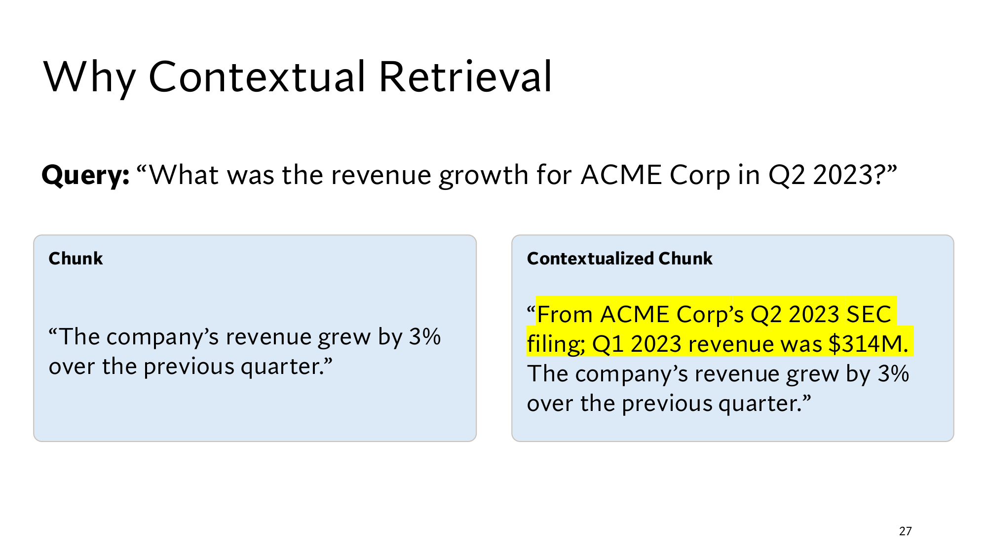
Take the example from the slides. The corpus holds the Q2 2023 quarterly filings of 50 companies, one per company. 50 companies is my example Almost every filing contains this line: The company’s revenue grew by X% over the previous quarter. The query is What was the revenue growth for ACME Corp in Q2 2023? ACME’s filing names the company and the quarter at the very top, so the chunk with the answer contains neither ACME nor Q2 2023.
Now count with lesson 2’s : how many of the query’s words also appear in the chunk. In lesson 2 the queue log scored 2, because it contained office and hour. After removing such as what, was, the, for and in, the query keeps 6 words: revenue, growth, ACME, Corp, Q2 and 2023. The ACME chunk contains only revenue, because it says grew, not growth. So it scores 1, and so do the other 49 chunks. my count
Think first
All 50 chunks score 1, and chunks with equal scores come out in random order. The retriever returns the top 20. How often does the ACME chunk make the top 20?
Show the answer
With a tie, the ACME chunk is equally likely to land in any of the 50 places. 20 of those places are in the top 20, so the chance is 20 ÷ 50 = 0.4, or 40%. The other 60% of the time the right chunk stays out of the top 20.
So the answer is in the corpus, yet the retriever misses it 60% of the time. An embedding does not save it either, because the embedding model reads only the chunk’s text. That text never mentions ACME, so the vector cannot carry anything about ACME.
Lesson 7’s keeps metadata with each chunk, but nobody will write metadata by hand for 60,000 chunks.
2Contextual retrieval: an LLM writes a context in front of each chunk
Contextual retrieval puts a short context in front of each chunk, written by an LLM that has read the whole document. Anthropic published the method in 2024. It runs four steps at , before any query arrives:
For each chunk, give the LLM the whole document and that chunk.
The LLM writes a short context for the chunk, 50 to 100 tokens long.
Put that context in front of the chunk. The new text is called a contextualized chunk.
Embed the contextualized chunk, and also add it to a word-based index, which comes in lesson 11.
For the ACME chunk, the LLM writes this context. The coloured part is the LLM’s, and the rest is the original chunk:
From ACME Corp’s Q2 2023 SEC filing; Q1 2023 revenue was $314M. The company’s revenue grew by 3% over the previous quarter.
Stanford’s slide: the query at the top, the bare chunk on the left, and the same chunk with the yellow context on the right. Click the image to open it at full size.
Think first
The query’s 6 words are revenue, growth, ACME, Corp, Q2 and 2023. What is the contextualized chunk’s word overlap score now? What will the other companies’ contextualized chunks score?
Show the answer
The ACME chunk scores 5: revenue, ACME, Corp, Q2 and 2023. Growth is still missing. The other companies’ contexts carry their own names, so they score at most 3: revenue, Q2 and 2023. my count
With the context added, the ACME chunk breaks out of the 49-way tie and goes straight to the top. The embedding model now also gets a text that contains ACME and Q2 2023.
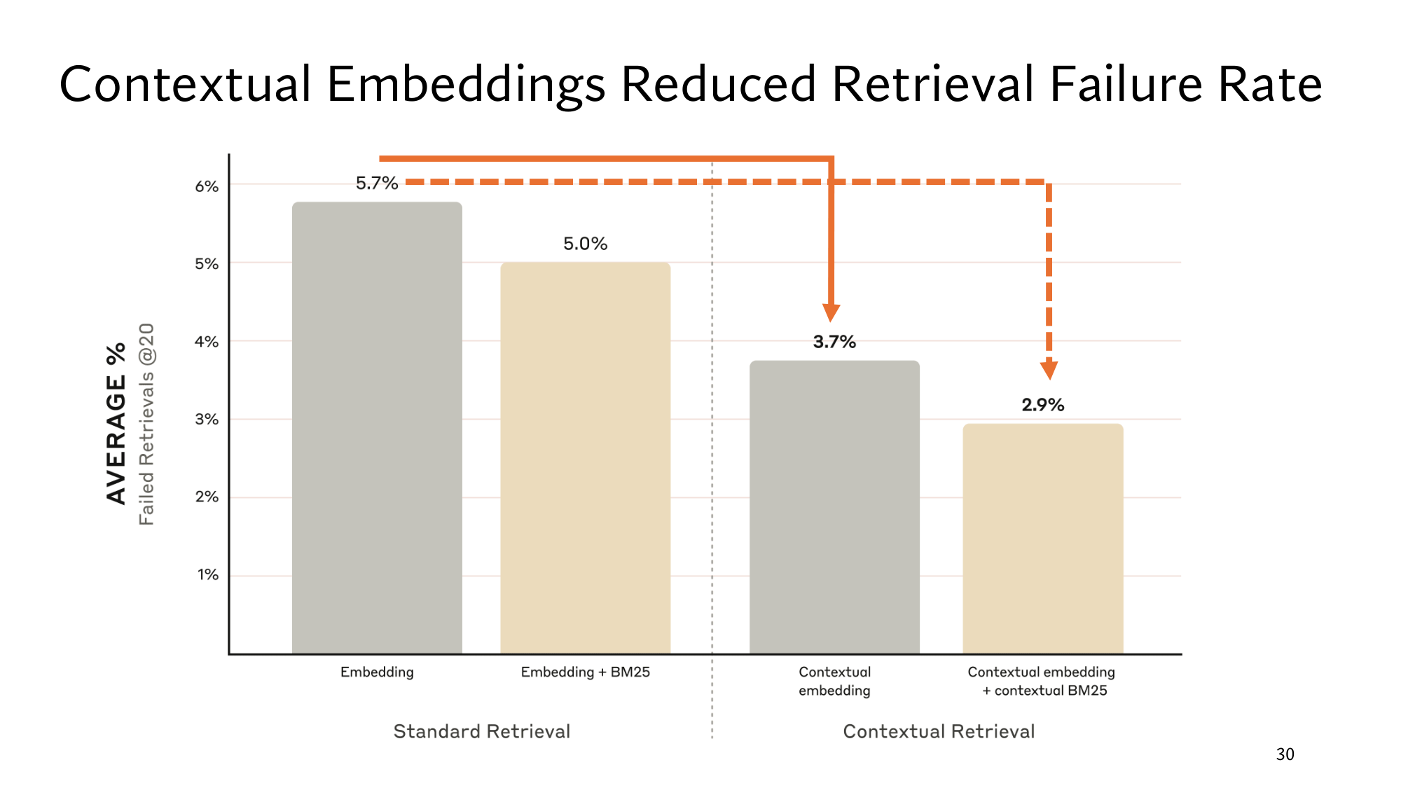
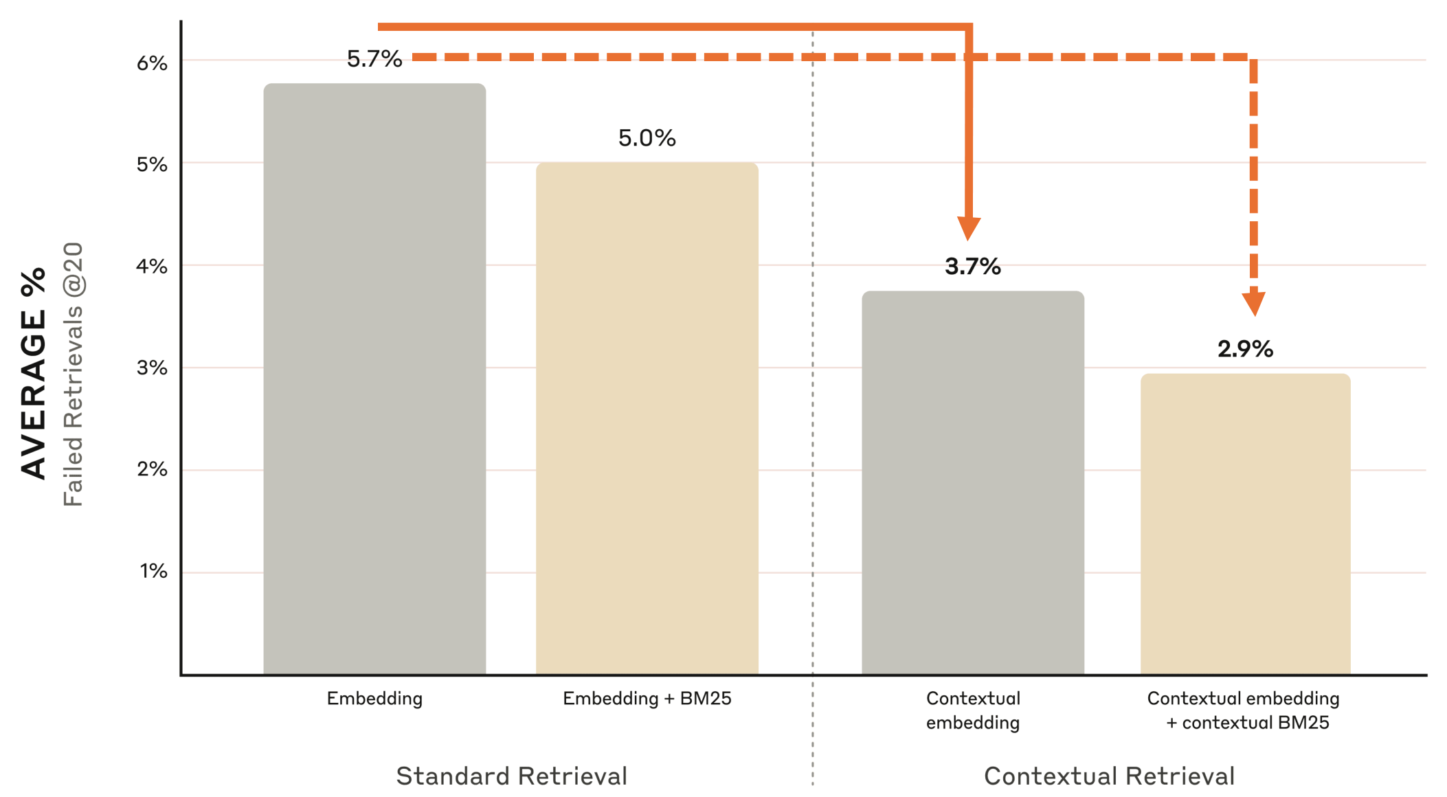
Anthropic’s results: failed retrievals@20
Anthropic measured the method on real data. Assume each query has one right chunk. Then failed retrievals@20 is the percentage of queries whose right chunk did not make the top 20. The smaller this number, the better.
The drop in the third row is easiest to see on 1,000 queries:
With plain chunks, 5.7% × 1,000 = 57 queries fail.
With contextualized chunks, 3.7% × 1,000 = 37 queries fail.
57 − 37 = 20 queries are saved, and 20 ÷ 57 = 0.35. So failures fell by 35%.
The failure rate fell by only 2 points, from 5.7 to 3.7, yet failures fell by 35%. The drop in points is 5.7 − 3.7, and the percentage drop divides that by the starting value, 5.7. Add the word-based index as well, and failures fall to 2.9%, which is (5.7 − 2.9) ÷ 5.7 = 0.49, about half. How to merge the two indexes’ lists comes in lesson 14.
The cost comes at indexing time: one LLM call per chunk, and the whole document in every call. With 60,000 chunks, that is 60,000 calls. There is no extra cost at query time, because the context is already in the index. There is also a risk: if the LLM writes a wrong context, that mistake stays in the index.
3Late chunking: encode the whole document first, then average each chunk
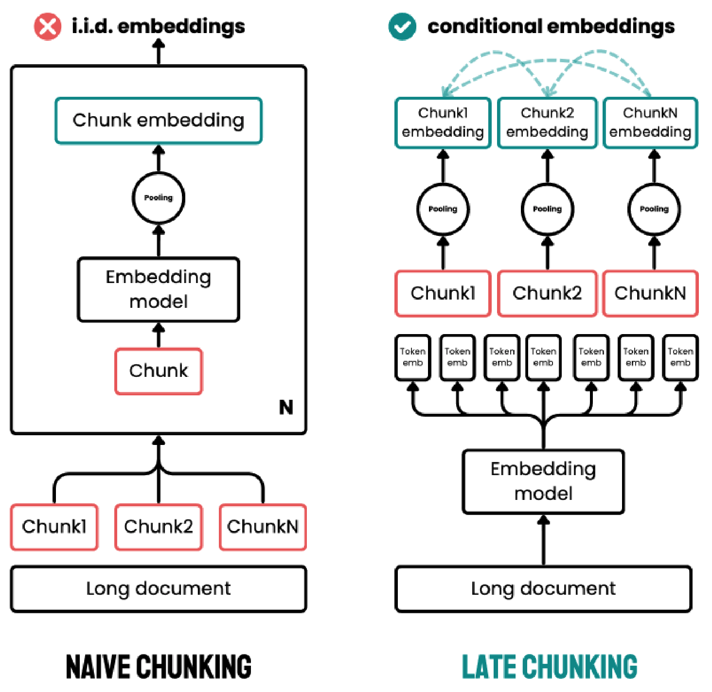
LLM calls are expensive, so the next question is whether the encoder alone can supply the context. Lesson 7’s builds each token’s vector from the words around it. There, late had the vector [0.1, 0.9] in one sentence and [0.9, 0.1] in the other. But the encoder only sees the text it is given.
The usual method gives the encoder only the chunk: cut first, then encode each chunk on its own. This is called naive chunking. The chunk’s tokens know nothing about the rest of the document.
Late chunking reverses the order: the encoder reads the whole document first, and the cutting happens afterwards.
Feed the whole document into a long-context encoder, an encoder that can read a very long text in one go, such as 8,192 tokens, about 10 pages. from the paper
The encoder returns a vector for every token, and every vector is built with the whole document in view.
Average the token vectors inside each chunk. That average is the chunk’s vector.
This average is lesson 7’s , for example [0.9, 0.1], [0.7, 0.3] and [0.8, 0.2] give [0.8, 0.2]. The cutting happens after encoding, that is, late, hence the name.
Take a small document: CS 329Z project milestone policy. It is due Week 6. The second chunk is It is due Week 6. In each vector, the first number says how much the text is about the project milestone, and the second how much it is about homework. my numbers
Token
Naive: chunk alone
Late: whole document
It
[0.5, 0.5]
[0.9, 0.1]
is
[0.5, 0.5]
[0.8, 0.2]
due
[0.6, 0.4]
[0.9, 0.1]
Week
[0.4, 0.6]
[0.9, 0.1]
6
[0.5, 0.5]
[1.0, 0.0]
Mean pooling
[0.5, 0.5]
[0.9, 0.1]
The last row works out like this:
Naive, first number: (0.5 + 0.5 + 0.6 + 0.4 + 0.5) ÷ 5 = 2.5 ÷ 5 = 0.5. The second number is also 0.5.
In the naive version, It cannot tell whether the text is about the milestone or about homework, so the vector sits in the middle. In the late version, the encoder also read the first sentence, so every token leans towards the milestone.
Take the query When is the project milestone due? with the vector [0.95, 0.05]. Lesson 3’s divides the dot product by the product of the two lengths, as in 0.74 ÷ (0.82 × 0.91) = 0.99. The cosine with the naive chunk takes three steps:
For the late chunk [0.9, 0.1], the same arithmetic gives 0.86 ÷ (0.951 × 0.906) = 1.00. The late chunk points almost exactly the way the query does, while the naive chunk stays at 0.74.
Think first
Now take a homework query with the vector [0.05, 0.95]. Work out its cosine with the naive chunk [0.5, 0.5] and with the late chunk [0.9, 0.1]. What weakness of the naive chunk shows up?
The naive chunk gives 0.74 for both queries, so the milestone chunk ranks just as high for the homework question. my query
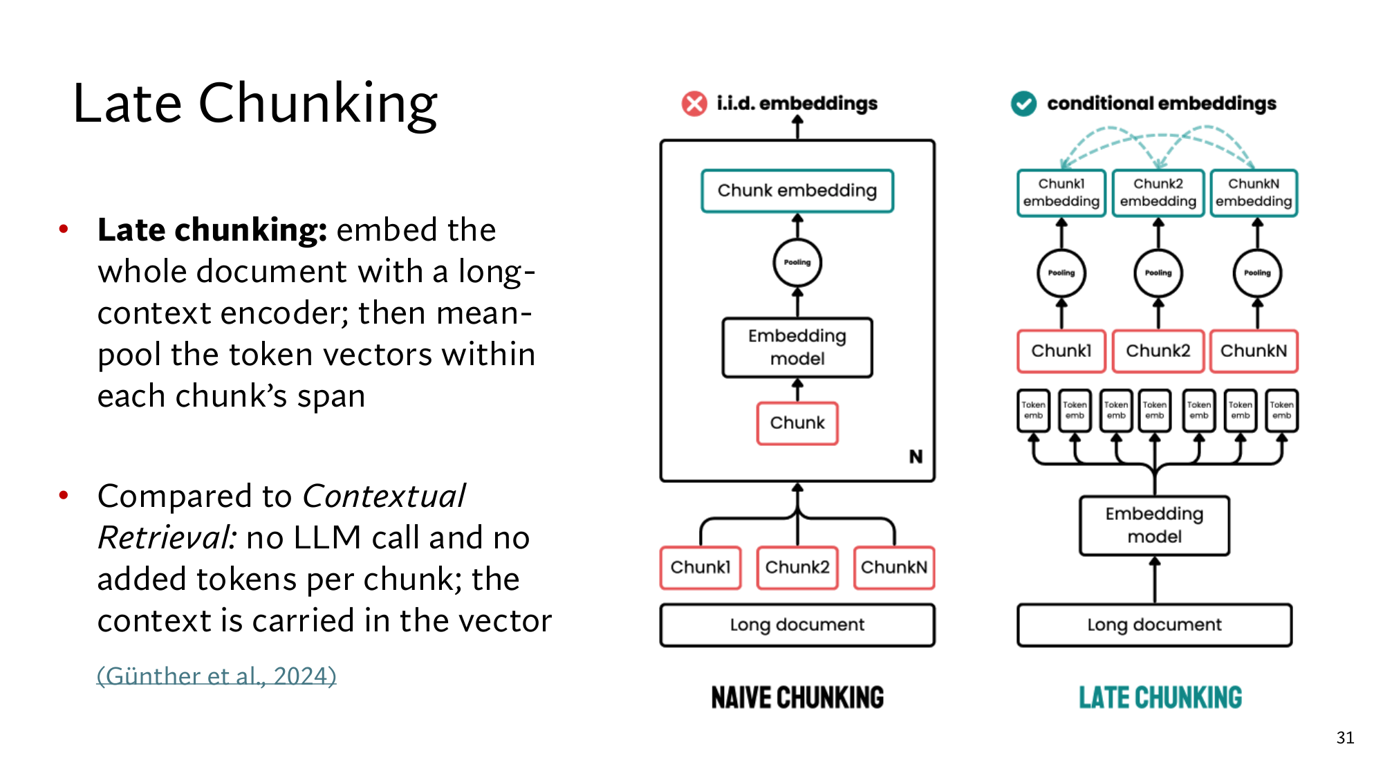
Stanford’s slide: naive chunking in the middle, and late chunking on the right.
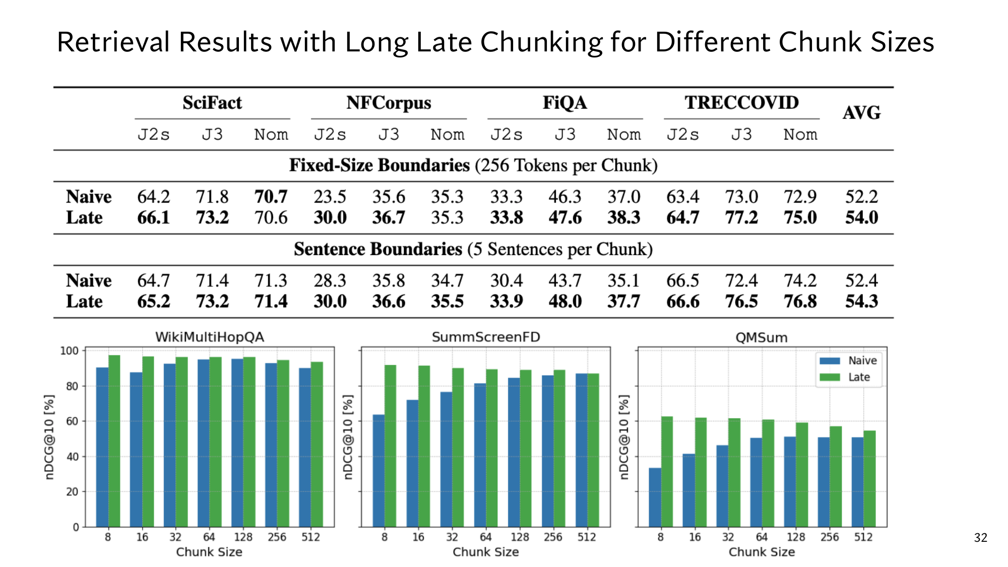
In the paper, with chunks of 256 tokens, late chunking raised the average score from 52.2 to 54.0. This is a ranking score from 0 to 100, which lesson 13 opens up. The gain is largest for the smallest chunks, because a small chunk loses the most context.
4Comparing the two methods: context in the text or in the vector
The two methods keep the context in different places: contextual retrieval writes it into the chunk’s text, and late chunking keeps it only in the vector. The other differences follow from this:
Contextual retrieval
Late chunking
Who supplies the context
An LLM, by writing text
The encoder, inside the vectors
Indexing cost
One LLM call per chunk
One encoder run per document
Does the chunk get longer?
Yes, by 50–100 tokens
No
Helps a word-based index
Yes, the new words are in the text
No
The ACME query shows the difference directly. After late chunking, the chunk’s text still does not contain ACME, so its word overlap score stays at 1. So only contextual retrieval helps a word-based index, while both help embeddings. Late chunking also has a limit: the whole document must fit within the encoder’s length limit, or the context gets cut again.
Think first
The corpus is very large, the budget for LLM calls is small, chunks are 64 tokens, and the retriever uses embeddings only. Which method do you pick? What if the retriever is a word-based index only?
Show the answer
Late chunking. It needs no LLM call, and its gain is largest on small chunks. On a word-based index alone, late chunking does nothing, because its context never reaches the text. Then pick contextual retrieval.
From here: the Stanford level
The 4 steps above are the same as in the easy version. The 5 steps below take you to the level of the Stanford slides: first Anthropic’s full pipeline and its numbers, then late chunking from the inside and the results of its paper, then both methods on the same example, and finally reading the slides yourself. Every piece of maths is explained where it first appears.
5Anthropic’s full pipeline: the diagram, the prompt, the cost and the metric
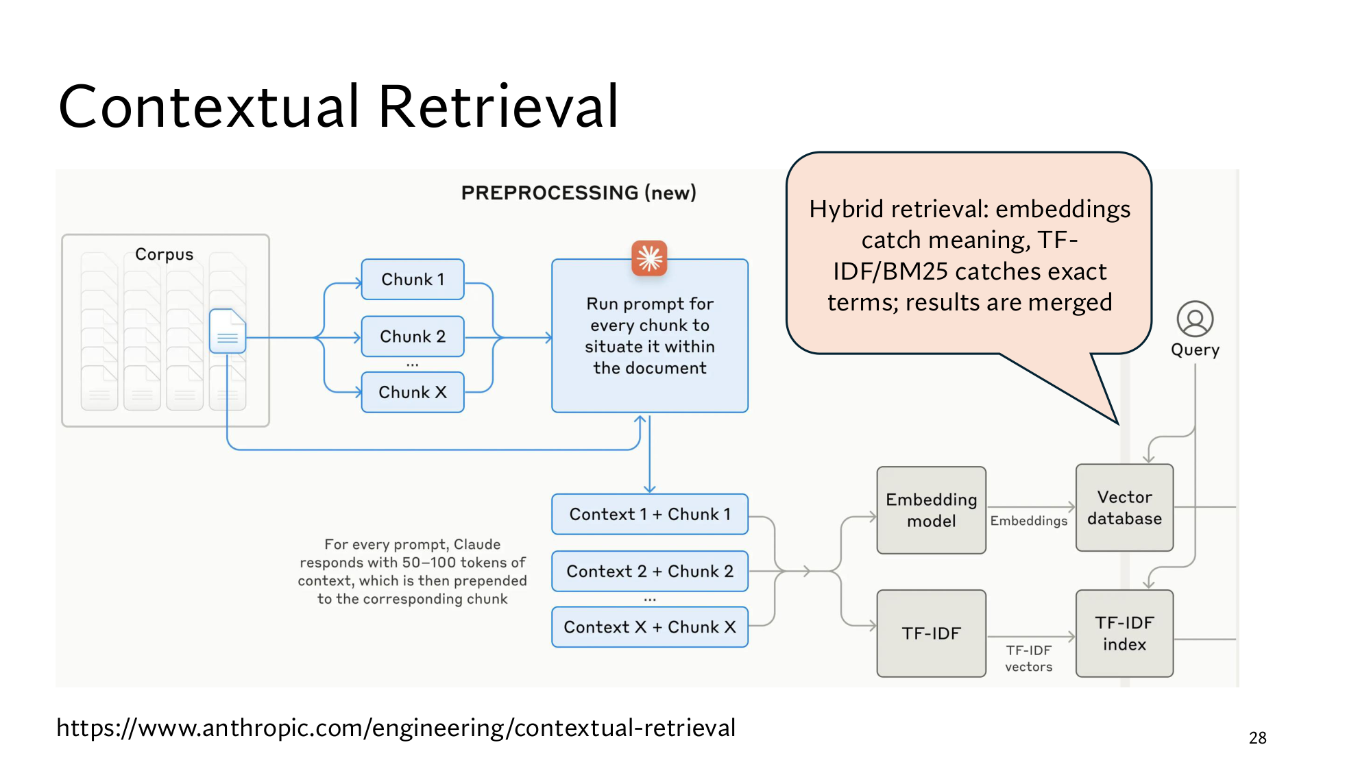
Step 2 gave the four steps of contextual retrieval. Stanford’s slide shows the same steps in a diagram from Anthropic, and this step reads every box in it. The numbers in this step come from Anthropic’s blog post Introducing Contextual Retrieval, and the slide’s diagram comes from the same post.
The diagram from Stanford’s contextual retrieval slide, enlarged. Click the image to open it at full size.
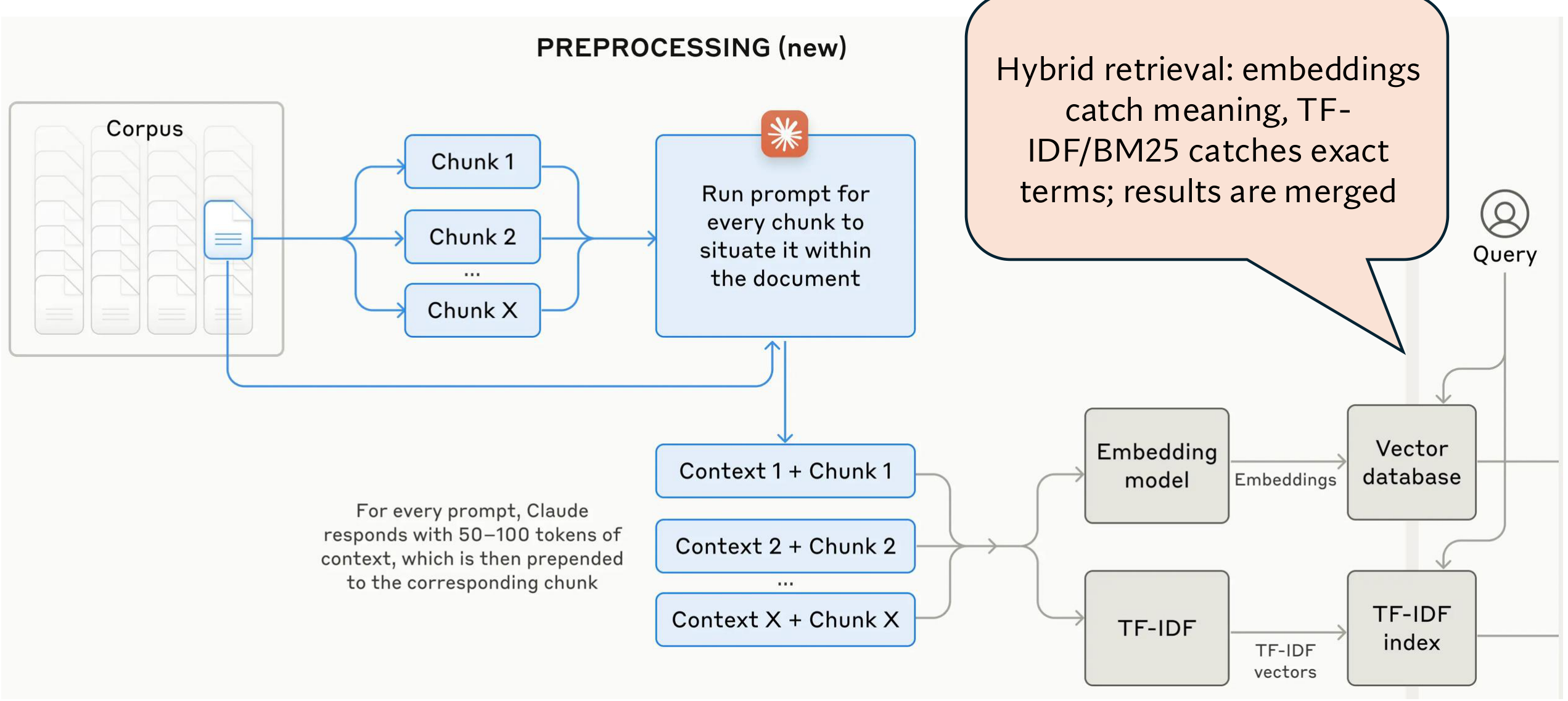
The diagram runs from left to right like this:
PREPROCESSING (new): this whole part runs at indexing time. New means a standard RAG pipeline does not have this step.
Corpus to Chunk 1 … Chunk X: one document from the corpus is cut into chunks. X is simply the number of chunks.
Run prompt for every chunk: one LLM call per chunk. The long blue line from below carries the whole document into this box, because the LLM needs the whole document along with the chunk.
Context 1 + Chunk 1: the LLM’s 50–100 token answer goes in front of the chunk. The slide calls this prepended.
Embedding model to Vector database: each contextualized chunk is embedded, and the embedding goes into a vector database.
TF-IDF to TF-IDF index: the same contextualized chunks also go into a word-based index.
Query: a query goes to both indexes. No LLM call happens at this point.
The box says TF-IDF, while the chart and the blog say BM25. multiplies each word’s count by a weight for how rare it is. For example, N = 6, n = 2 and f = 2 give 2 × ln 3 = 2.20. is an improved form of the same idea that caps the benefit of repeated words and lowers the weight of long passages. The blog’s index is a BM25 index, and the blog calls it Contextual BM25. from the blog
The callout at the top says that embeddings catch meaning, TF-IDF/BM25 catches exact words, and the system merges the results of both. Merging the lists of two retrievers is called . For example, BM25’s list E1, E3, E2 and the dense list E2, E1, E3 become one list. The blog merges the two lists with rank fusion, which comes in lesson 14. from the blog
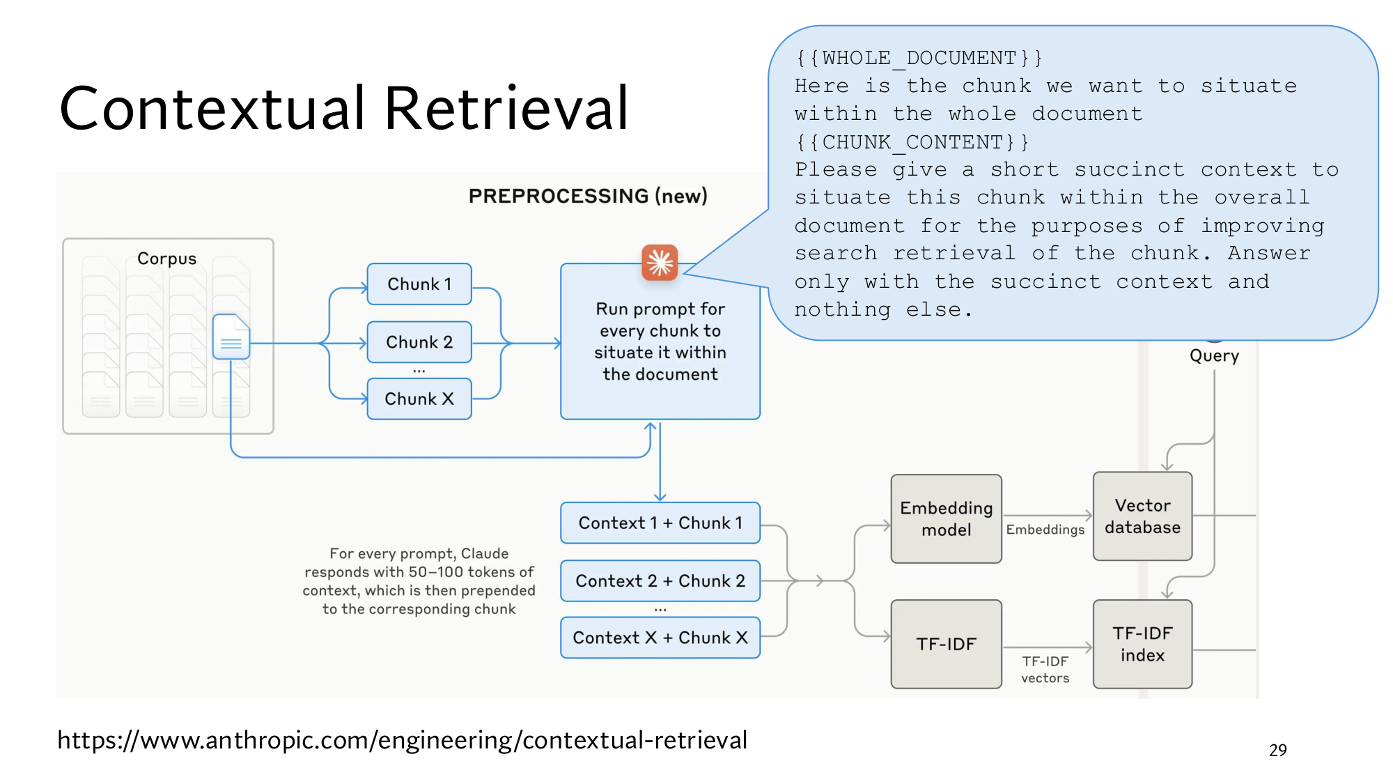
The prompt, line by line
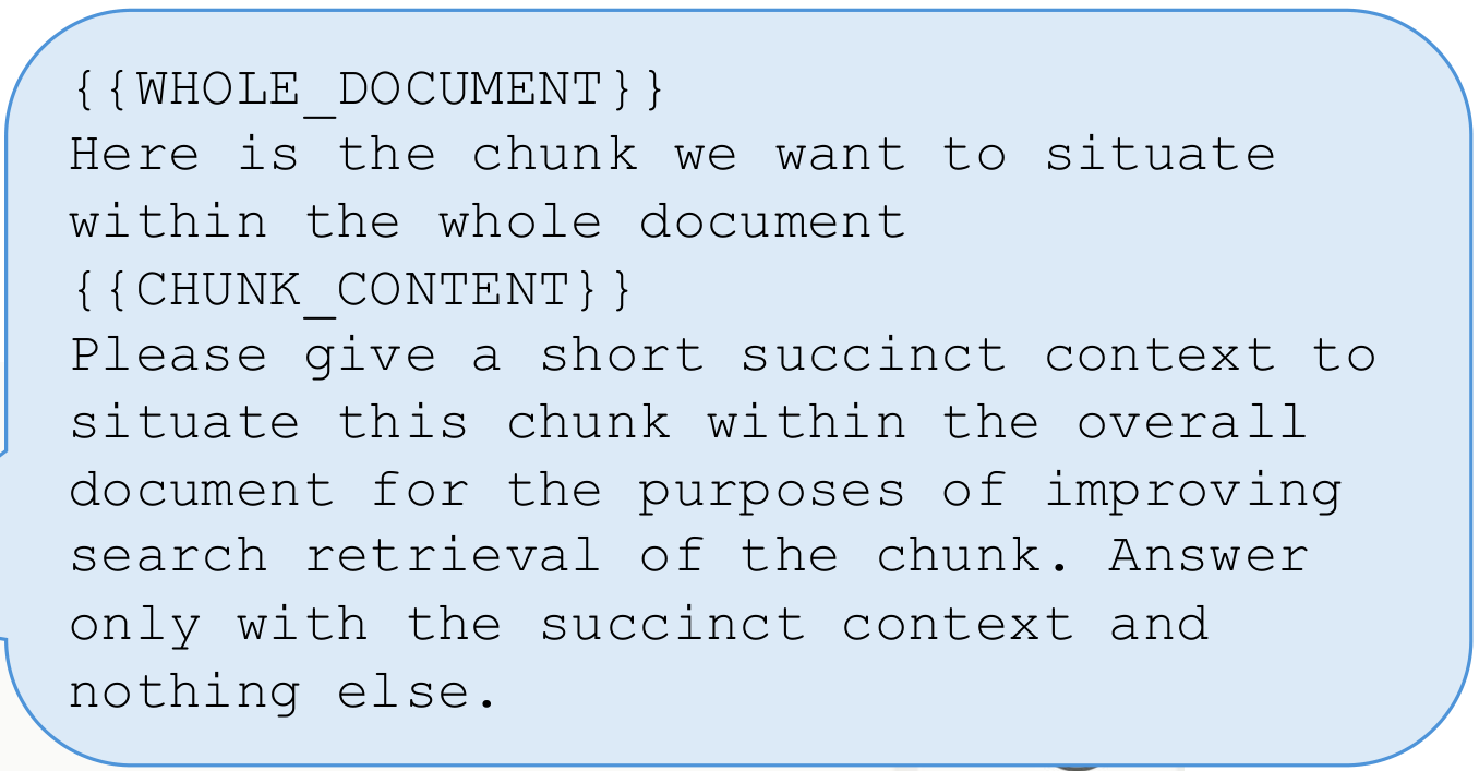
The LLM prompt on Stanford’s slide, enlarged.
The prompt has four parts. {{WHOLE_DOCUMENT}} is a placeholder, an empty slot that the program fills with the whole document on every call. Then a line says that what follows is the chunk to be placed within the document. The program fills {{CHUNK_CONTENT}} with that chunk. The last part asks the LLM for a short context for search, and says the answer must contain nothing else.
That last condition matters, because the program puts the LLM’s whole answer, unchanged, in front of the chunk. If the LLM wrote a line like Sure, here is the context:, that line would go into the index with every chunk. In the blog’s prompt, the document sits inside <document> tags and the chunk inside <chunk> tags, which the slide does not show. Anthropic ran this prompt on Claude 3 Haiku. from the blog
The cost of the LLM calls, and prompt caching
Step 2 gave the cost in one line: one call per chunk, and the whole document in every call. Here is the count under the blog’s assumptions: chunks of 800 tokens, documents of 8,000 tokens, 50 tokens of instructions, and 100 tokens of context per chunk. from the blog
One document has 8,000 ÷ 800 = 10 chunks, so 10 LLM calls.
In each call the LLM reads 8,000 + 800 + 50 = 8,850 tokens.
All ten calls together read 10 × 8,850 = 88,500 tokens, which is 88,500 ÷ 8,000 = about 11 times the document’s length.
The LLM writes 100 tokens per call, so 10 × 100 = 1,000 tokens. my arithmetic
The biggest part of step 3 is the same document, repeated in all ten calls. Prompt caching makes exactly this repetition cheap. The LLM service keeps one part of the prompt after the first call, here the whole document. Later calls do not pay the full price to read it again. According to the blog, the whole cost then comes to $1.02 per million document tokens. from the blog
The index grows too. If a chunk of 800 tokens gets 100 tokens of context, then 100 ÷ 800 = 0.125, so every chunk becomes 12.5% longer. my arithmetic
The blog makes two more points. If the whole knowledge base is under 200,000 tokens, about 500 pages, put it straight into the prompt, and you need no RAG. The second point ties back to lesson 7: adding one generic summary of the document to each chunk gave very little gain. from the blog
The chart’s metric, the average, and reranking
The chart’s y-axis says AVERAGE % and Failed Retrievals @20. The blog calls its metric 1 minus recall@20: the percentage of relevant documents that were not retrieved within the top 20 chunks. from the blog Lesson 13’s is right chunks found in the top k ÷ all right chunks, for example 1 found out of 2 gives 0.5. When each query has only one right chunk, 1 − Recall@20 is the same as lesson 13’s , that is, 1 − Hit@20.
AVERAGE means each bar is an average over four kinds of data: codebases, fiction, ArXiv papers and science papers. The embedding model was the best one in their tests, Gemini Text 004, and they looked at the top 20 chunks per query. from the blog According to the blog, adding context improved results for every embedding model and every kind of data they tried.
The chart has two halves. On the left is Standard Retrieval, with plain chunks, and on the right Contextual Retrieval, with contextualized chunks. In each half, the first bar is embeddings alone, and the second is embeddings plus BM25. The third bar is labelled Contextual embedding, and here that means the embedding of a contextualized chunk, not lesson 7’s token-level .
Step 2 gave the rule for a percentage drop: (old − new) ÷ old. The blog adds one more step. Lesson 6’s is a slow but precise model that sorts a returned list again. Anthropic first took the top 150 chunks, sorted them again with Cohere’s reranker, and kept the top 20. from the blog
Method
Failed@20
Points down
% down
Plain chunks, embedding
5.7
–
–
Plain chunks, embedding + BM25
5.0
0.7
12%
Contextualized, embedding
3.7
2.0
35%
Contextualized, embedding + BM25
2.9
2.8
49%
The row above + reranking
1.9
3.8
67%
Every row is compared with 5.7. For the last row: (5.7 − 1.9) ÷ 5.7 = 3.8 ÷ 5.7 = 0.67. The blog also tried giving the model 5, 10 and 20 chunks, and 20 worked best. from the blog
Think first
With plain chunks, embedding + BM25 had a failure rate of 5.0%, and with contextualized chunks 2.9%. By what percentage did adding context cut the failures of the BM25 system?
Show the answer
(5.0 − 2.9) ÷ 5.0 = 2.1 ÷ 5.0 = 0.42, or 42%. The blog’s 49% starts from 5.7, and this 42% starts from 5.0. A percentage drop always depends on which number you compare with. my arithmetic
6Late chunking from the inside: conditional embeddings, attention and the pooling formula
Step 3 showed the result of late chunking: the vector of It became [0.9, 0.1] instead of [0.5, 0.5]. This step shows how the encoder does that, and how the paper writes it as a formula.
i.i.d. and conditional embeddings
On the slide’s diagram, the naive half is labelled i.i.d. embeddings and the late half conditional embeddings. i.i.d. is a statistics term, short for independent and identically distributed. Here it means that every chunk’s vector comes from the same model, completely separately from the other chunks, that is, independently.
Conditional comes from lesson 4’s , where p(A | B) meant the probability of A once B is known, for example p(full | Tuesday) = 0.80. In late chunking, each chunk’s vector is conditional on the whole document: it is built with the document known. The dashed arrows between the chunk embeddings on the diagram show exactly this: every chunk’s vector is affected by the other chunks.
The naive box has an N in its corner. It means the box runs N times, once per chunk, and each time the model sees only one chunk. In late chunking the model runs once, and the small Token emb boxes are the vectors of the individual tokens.
How a token gets to see the whole document
Inside the encoder, each token’s vector is updated from the vectors of the other tokens, and does this. For each token, attention takes a weighted average of the other tokens’ vectors. In a weighted average you multiply each vector by its weight and add the results, and the weights add up to 1.
Suppose the starting vector of It is [0.5, 0.5] and that of milestone is [1.0, 0.0]. Attention gives milestone a weight of 0.8, and It itself 0.2. my numbers
That is the late [0.9, 0.1] from the table in step 3. In naive chunking, milestone is not inside the chunk at all. Then It can only average over It, is, due, Week and 6, and they all sit in the middle. A real encoder does this over many layers, and the model works out the weights itself.
The paper shows the same effect with a real encoder. It cut the Wikipedia article on Berlin into sentences and computed the cosine between each sentence’s vector and the vector of the word Berlin. The model was jina-embeddings-v2-small. from the paper
Sentence
Naive
Late
Berlin is the capital and largest city of Germany…
0.8486
0.8495
Its more than 3.85 million inhabitants…
0.7084
0.8249
The city is also one of the states of Germany…
0.7535
0.8498
The first sentence names Berlin, so both methods give almost the same cosine. The second and third sentences only say Its and The city. There, late chunking lifts the cosine from 0.7084 to 0.8249, and from 0.7535 to 0.8498.
The paper’s pooling formula
The paper writes late chunking as an algorithm. A chunker cuts the text into chunks, measured in characters. A tokenizer turns the text into tokens and gives each token’s length in characters. The model returns a vector for every token, which the paper writes as ϑ: ϑ1 to ϑm, where m is the number of tokens. from the paper
The algorithm then walks through the tokens one by one, adding up their lengths in characters. When the total reaches the chunk’s length, the chunk ends there. This gives the position of each chunk’s first and last token, which the paper writes as cuestart and cueend. Each chunk’s vector is then:
ei = ∑j = cuestartcueend ϑj(cueend + 1) − cuestart
The is from lesson 3: keep adding from the position written below to the one written above, as in a1b1 + a2b2. Now run it on our document, treating every word as one token and leaving out the full stops. my simplification Then CS to policy are tokens 1 to 5, and It to 6 are tokens 6 to 10.
For chunk 2, cuestart = 6 and cueend = 10.
The sum on top, for the first number: ϑ6 to ϑ10 give 0.9 + 0.8 + 0.9 + 0.9 + 1.0 = 4.5.
Below: (10 + 1) − 6 = 5, the number of tokens in the chunk. The +1 is there because counting from 6 to 10 includes both 6 and 10.
The first number of e2: 4.5 ÷ 5 = 0.9, the late number from step 3.
Naive chunking takes the same average. The only difference is in ϑ: in naive chunking, ϑ6 to ϑ10 come from a run in which the model read only chunk 2. The model also adds special tokens such as [CLS] at the start of the text and [SEP] at the end, which belong to no word. The paper puts their vectors into the average of the first and last chunk. from the paper
Late chunking does not require training the model again. According to the paper, it works with any long-context embedding model that uses mean pooling, and with any chunking method. from the paper
7The paper’s results: the table, chunk size and long late chunking
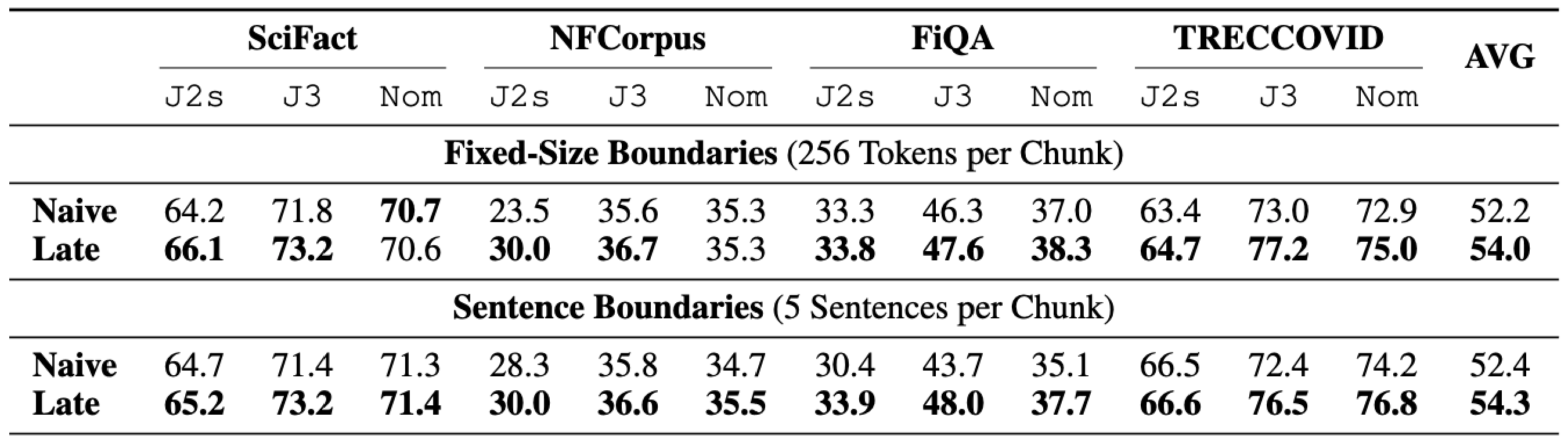
Stanford’s last slide in this part shows two results from the paper: a table at the top and three charts below. Both use the score , which comes in lesson 13. nDCG@10 checks how high the right chunks sit in the top 10, and it lies between 0 and 1, for example 2.5 ÷ 3.631 = 0.689. The paper multiplies it by 100 and writes it as a percentage, so a score of 0.689 would appear as 68.9. the slide prints nDCG@10 only on the charts, and the table’s metric is from the paper
The table: 4 datasets and 3 models
The table’s columns cover 4 datasets: SciFact, NFCorpus, FiQA and TRECCOVID. These are small datasets from a benchmark called BeIR, ready-made sets of queries, documents and right answers. Under each dataset are 3 embedding models: J2s is jina-embeddings-v2-small, J3 is jina-embeddings-v3, and Nom is nomic-embed-text-v1. from the paper
The rows use two kinds of boundaries: chunks of 256 tokens each, and chunks of 5 sentences each. In each pair, naive is on top and late below, and the bold number is the larger of the two. The AVG column is a plain average of 12 numbers: add all twelve and divide by 12. For the fixed-size rows: my arithmetic
Naive average: 627.0 ÷ 12 = 52.25, which the table writes as 52.2.
The late sum is 648.5, and 648.5 ÷ 12 = 54.04, so 54.0.
So on average late chunking is ahead by 54.04 − 52.25 = 1.79, about 1.8 points. As a percentage that is 1.79 ÷ 52.25 = 0.034, an improvement of about 3.4%. In the sentence rows, the average went from 52.4 to 54.3, about 1.9 points.
In the 12 fixed-size pairs, late chunking is ahead 10 times. On SciFact with Nom it is slightly behind, 70.6 against 70.7, and on NFCorpus with Nom the two tie at 35.3. The biggest gain is on NFCorpus with J2s: 23.5 to 30.0, or 6.5 points. According to the paper, NFCorpus has long documents. from the paper A long document gets cut into more chunks, so each chunk loses more context there.
The paper has a third pair of rows that is not on the slide: semantic sentence boundaries, which put similar sentences into one chunk. There too the average went from 52.4 to 53.8. The paper also tested lesson 7’s . With overlap, a new chunk repeats the last few tokens of the previous one, for example 6 words for a date of 7 words. An overlap of 16 tokens on chunks of 256 tokens neither clearly helped nor hurt. from the paper
The three chunk-size charts
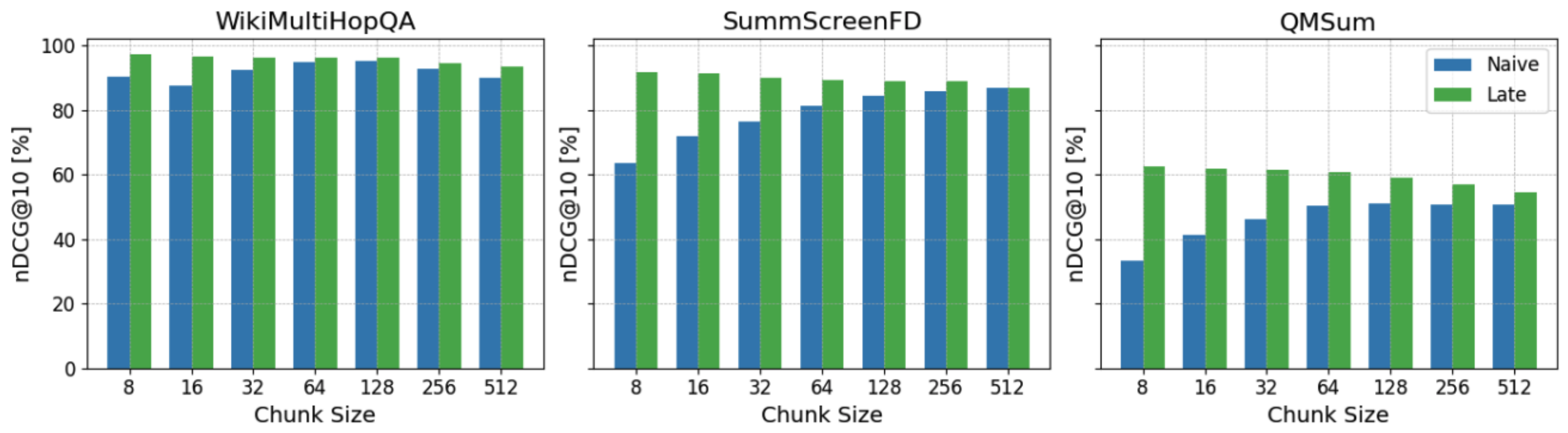
The three charts below have chunk size on the x-axis: 8, 16, 32, 64, 128, 256 and 512 tokens. Each size is double the one before. The y-axis is nDCG@10, in percent. Blue bars are naive, and green bars are late.
The three datasets, WikiMultiHopQA, SummScreenFD and QMSum, come from a benchmark called LongEmbed, which has reading comprehension questions over long documents. The model was J2s. from the paper Reading exact numbers off charts is unreliable, so look at their shape instead:
In every chart, the green bar is clearly above the blue one for small chunks.
On SummScreenFD and QMSum, the blue bars rise as chunks grow, while the green bars stay roughly level, so the gap shrinks. On WikiMultiHopQA, both colours are high at every size.
On SummScreenFD, the two bars at 512 tokens are about equal. On QMSum, the blue bar at 8 tokens is the lowest, and that is where the gap is largest.
Naive chunking gets context only when the chunk itself is big. Late chunking gets its context from the whole document, whatever the chunk size.
Long late chunking: when a document is longer than the encoder’s limit
The slide’s title says Long Late Chunking. Recall the limit from step 4: the document must fit within the encoder’s limit. Many LongEmbed documents are longer than J2s’s limit of 8,192 tokens. For these the paper introduces long late chunking. Read the document in large windows of lmax tokens, and start each new window by repeating the last ω tokens of the previous one. from the paper
Suppose a document has 20,000 tokens, lmax = 8,192 and ω = 1,000. my choice of ω and document
The first window reads tokens 1 to 8,192.
The second window starts 1,000 tokens back, at token 7,193, reads 8,192 tokens and stops at 15,384.
The third window starts at 14,385 and runs to the end of the document, token 20,000.
The first 1,000 tokens of the second window only provide context, and their vectors stay the ones from the first window. This way, the vector of token 8,193 is also built with the 1,000 tokens before it in view. The slide’s charts use this long late chunking. According to the paper, that is why the scores here are higher than in an earlier experiment, where the paper cut documents off at 8,192 tokens. from the paper
Where late chunking did not help
The paper finds two weak spots. On some reading comprehension datasets with large chunks, naive chunking did better. The paper’s guess is that the answer there is one specific sentence hidden in unrelated text. In the synthetic datasets Needle-8192 and Passkey-8192, a short useful fact sits inside unrelated text, and the surrounding context is of no use at all. from the paper
So late chunking helps only when the surrounding text really tells you what the chunk means. The company name in ACME’s filing is that kind of text. The paper also shows that chunking pays off even with a long-context model. On NarrativeQA with J2s, nDCG@10 was 32.73 without chunking at 8,192 tokens, and 47.63 with chunks of 512 tokens. from the paper This is lesson 7’s point: a lot of text blurs together in one vector.
8Both methods on the same ACME example
The paper compared late chunking with contextual retrieval in a small experiment, using the same ACME example. A made-up financial document has 5 chunks. The query is What is ACME Corp’s revenue growth for Q2 2023?, worded slightly differently from the slide’s query. The right chunk is It highlighted a 3% revenue growth over the previous quarter., which does not name the company. from the paper
The paper computed the cosine of each chunk with the query in three ways. For contextual retrieval, Claude 3 Haiku wrote a context in front of each chunk, and all three methods used the embedding model jina-embeddings-v2-small-en. from the paper
Chunk
Naive
Late
Contextual
1The recent SEC filing provided insights into ACME Corp’s performance for Q2 2023.
0.8505
0.8305
0.8069
2, the right chunkIt highlighted a 3% revenue growth over the previous quarter.
0.6343
0.8516
0.8590
3The company, which had a revenue of $314 million in the prior quarter, showed steady progress.
0.6169
0.8424
0.8546
4They attributed this growth to strategic initiatives…
0.5191
0.7997
0.8234
5The report emphasized the company’s resilience…
0.6007
0.8022
0.8061
Think first
If the retriever returns the one chunk with the largest cosine, which chunk comes back for each method? Where does the right chunk stand under naive chunking?
Show the answer
Naive returns chunk 1, with 0.8505, because it names ACME Corp and Q2 2023 but has no growth figure. The right chunk is second, with 0.6343. Late puts the right chunk on top with 0.8516, and contextual with 0.8590.
In both methods the right chunk’s cosine is about 0.85. The paper’s conclusion is that the two methods give nearly the same scores, and late chunking needs no extra LLM. This is a small experiment on one document, so it does not settle which method wins on a large corpus.
In the contextual chunks, the LLM’s context can add words like ACME and Q2 2023, so a word-based index could also find the right chunk there. Late chunking leaves the chunk’s text unchanged, as step 4 showed.
The paper also offers a training method called span pooling. During training, the document’s vector is the average of only the tokens in the answer span. This teaches the model to pack useful nearby information into each token. The loss is like lesson 12’s , where scores 1.0, 2.0 and 1.5 gave a loss of 1.68. This training gave a small but consistent gain. from the paper
9Now read Stanford’s slides yourself
Below are all six Stanford slides of this part, unchanged. Under each slide are a few questions. Think of the answer first, then open it. If something stops you, go back to the step named in the answer. If a slide looks small on a phone, click the image to open it at full size.
Stanford’s slide: Why Contextual Retrieval.
Read the first slide
How many of the query’s 6 words does the chunk on the left contain, and why is this chunk hard for a retriever?
Show the answer
Only revenue, so it scores 1. All 50 companies’ filings contain this line, so all 50 chunks tie, and the chance of making the top 20 is 40%. (Step 1)
Who wrote the yellow part, and where did it get ACME and Q2 2023 from?
Show the answer
The LLM, using the contextual retrieval prompt. It got the whole document along with the chunk, and the company name and quarter were at the top of that document. (Steps 2 and 5)
The yellow part says Q1 2023 revenue was $314M. What does that make Q2 2023 revenue?
Show the answer
Revenue grew by 3%. 3% of 314 is 314 × 0.03 = 9.42, and 314 + 9.42 = 323.42, about $323M. The context also gave the chunk information the answer writer needs. my arithmetic (Step 2)
Stanford’s slide: Contextual Retrieval, with the hybrid retrieval callout. Its diagram is enlarged in step 5.
Read the pipeline slide
What does the long blue line from the corpus to the prompt box carry?
Show the answer
The whole document. The LLM needs the whole document with each chunk, or it cannot tell what the chunk is about. (Step 5)
The callout says results are merged. Which results, and what does merging them buy you?
Show the answer
The lists from the vector database and from the TF-IDF/BM25 index. Embeddings catch meaning and BM25 catches exact words, so on contextualized chunks failures fall from 3.7% to 2.9%. (Steps 2 and 5)
How many LLM calls does a query need?
Show the answer
None. The LLM runs only during PREPROCESSING, and the query goes straight to both indexes. (Steps 2 and 5)
Stanford’s slide: the same pipeline, with the LLM prompt on top. The prompt is enlarged in step 5.
Read the prompt slide
What are {{WHOLE_DOCUMENT}} and {{CHUNK_CONTENT}}?
Show the answer
Both are placeholders, empty slots. On every call the program fills the first with the whole document and the second with the chunk. (Step 5)
Why does the prompt end with Answer only with the succinct context and nothing else?
Show the answer
The LLM’s whole answer goes in front of the chunk unchanged. Any other line in the answer would go into the index with every chunk. (Step 5)
A document of 8,000 tokens has chunks of 800 tokens, and the instructions are 50 tokens. Without caching, how many tokens does this prompt read in total?
Show the answer
10 calls, each reading 8,000 + 800 + 50 = 8,850 tokens, so 88,500 in total, about 11 times the document. Prompt caching makes this repetition cheap. (Step 5)
Stanford’s slide: Contextual Embeddings Reduced Retrieval Failure Rate, and below it the chart, enlarged.
Read the chart slide
What is each bar an average of, and what is the metric on the y-axis?
Show the answer
An average over four kinds of data, codebases, fiction, ArXiv papers and science papers, with Gemini Text 004 embeddings. The metric is failed retrievals@20, which the blog calls 1 minus recall@20. (Step 5)
Which two drops do the solid and dashed orange arrows show?
Show the answer
The solid arrow goes from 5.7 to 3.7, a drop of (5.7 − 3.7) ÷ 5.7 = 35%. The dashed arrow goes from 5.7 to 2.9, a drop of 49%. (Step 2)
The title says Contextual Embeddings. Does contextual embedding mean the same as in lesson 7 here?
Show the answer
No. Here it means the embedding of a contextualized chunk, the vector of a text with the LLM’s context in front of it. Lesson 7’s contextual embedding is a token’s vector that depends on its sentence. (Step 5)
Stanford’s slide: Late Chunking, and below it the diagram, enlarged.
Read the late chunking slide
What do the labels i.i.d. embeddings and conditional embeddings on the diagram mean?
Show the answer
i.i.d.: each chunk’s vector is built completely separately from the other chunks. Conditional: each chunk’s vector is built with the whole document in view, and the dashed arrows show that influence. (Step 6)
Why is there an N in the corner of the naive box, and how many times does the model run in late chunking?
Show the answer
There are N chunks, so in naive chunking the model runs N times, once per chunk. In late chunking the model runs once per document. (Steps 3 and 6)
The second bullet on the left says no LLM call and no added tokens per chunk, and then the context is carried in the vector. What does that mean for a word-based index?
Show the answer
The chunk’s text does not change, so BM25 never sees ACME, and the ACME chunk’s word overlap score stays at 1. (Step 4)
Stanford’s slide: Retrieval Results with Long Late Chunking for Different Chunk Sizes, and below it the table and the charts, enlarged.
Read the results slide
What are J2s, J3 and Nom in the table, and how was the fixed-size late row’s AVG of 54.0 computed?
Show the answer
They are three embedding models. 54.0 is the average of the late row’s 12 numbers: 648.5 ÷ 12 = 54.04. (Step 7)
Where in the table is late chunking not ahead of naive chunking?
Show the answer
In the fixed-size rows, on SciFact with Nom, 70.6 against 70.7, and on NFCorpus with Nom, where both are 35.3. In the sentence rows, late is ahead everywhere. (Step 7)
Where is the gap in the charts largest, and what does Long in the title mean?
Show the answer
At the smallest chunks, because that is where naive chunking gets the least context. Long means long late chunking: reading documents longer than the encoder’s limit in overlapping windows. (Step 7)
3 points from this lesson
Cutting makes a chunk lose its context. The ACME chunk ended up tied with 49 other chunks, and it makes the top 20 only 40% of the time.
Contextual retrieval has an LLM write a context in front of each chunk. Failed retrievals@20 fell from 5.7% to 2.9%, and to 1.9% with reranking, a 67% drop. The cost comes at indexing time: without caching, the LLM reads about 11 times as many tokens as the document has.
Late chunking builds conditional vectors from the whole document, then averages each chunk. In the paper the average score rose from 52.2 to 54.0, with the largest gain on small chunks. In the ACME test, both methods put the right chunk on top.
New terms in this lesson
Context loss
After cutting, a chunk can no longer say which document or topic it belongs to. For example, The company’s revenue grew by 3% does not name the company.
Contextual retrieval
Indexing each chunk with a 50–100 token context, written by an LLM, placed in front of it. For example, adding From ACME Corp’s Q2 2023 SEC filing.
Failed retrievals@20
When each query has one right chunk, the percentage of queries whose right chunk is not in the top 20. Smaller is better. For example, 29 failures in 1,000 queries is 2.9%.
Naive chunking
Cutting first, then encoding each chunk on its own. Then the vector of It is due Week 6 stays at [0.5, 0.5].
Late chunking
Encoding the whole document first, then mean pooling each chunk’s token vectors. Then the vector of It is due Week 6 becomes [0.9, 0.1].
Long-context encoder
An encoder that can read a very long text in one go. For example, 8,192 tokens, about 10 pages.
Prompt caching
The LLM service keeps a repeated part of the prompt after the first call, such as the whole document, so that part is cheap in later calls. According to the blog, contextual retrieval then costs $1.02 per million document tokens.
i.i.d. and conditional embeddings
i.i.d.: each chunk’s vector is built completely separately from the other chunks, as in naive chunking. Conditional: each chunk’s vector is built with the whole document in view, as in late chunking, where It gets [0.9, 0.1].
Long late chunking
Late chunking for a document longer than the encoder’s limit, read in large overlapping windows. For example, 20,000 tokens read in windows of 8,192 tokens, each new window starting 1,000 tokens back.