The moment you cut a document into chunks, each chunk loses the text around it, and that text often said what the chunk was about. This lesson teaches two ways to give that context back. In contextual retrieval, an LLM writes a short context for each chunk. In late chunking, the encoder reads the whole document first.
In lesson 7, the queue log chunk office hour averaged 3. did not say which day it was about. This lesson looks at the same problem in the filings of 50 companies.
The ladder for this lesson
The ladder has 4 steps. Under each step you can see what you will be able to do after it.
Context lossCount your way to why the ACME chunk makes the top 20 only 40% of the time.
Contextual retrievalExplain how the score goes from 1 to 5, and what it means that failures drop from 5.7% to 2.9%.
Late chunkingCompute naive and late chunk vectors by hand, and show the difference with cosine.
What you need first: Lesson 2 (word overlap), Lesson 3 (embedding, cosine) and Lesson 7 (chunk, contextual embedding, mean pooling). If you already know a step, skip to the next one. A word with a dotted underline and ▾ opens its definition when you click it.
1Context loss: after cutting, a chunk no longer says what it is about
Context loss means that after cutting, a chunk no longer contains the words that say what it is about. A is the piece of a document that a retriever returns. A name often appears once, at the top of a document, so the chunks further down are left without it.
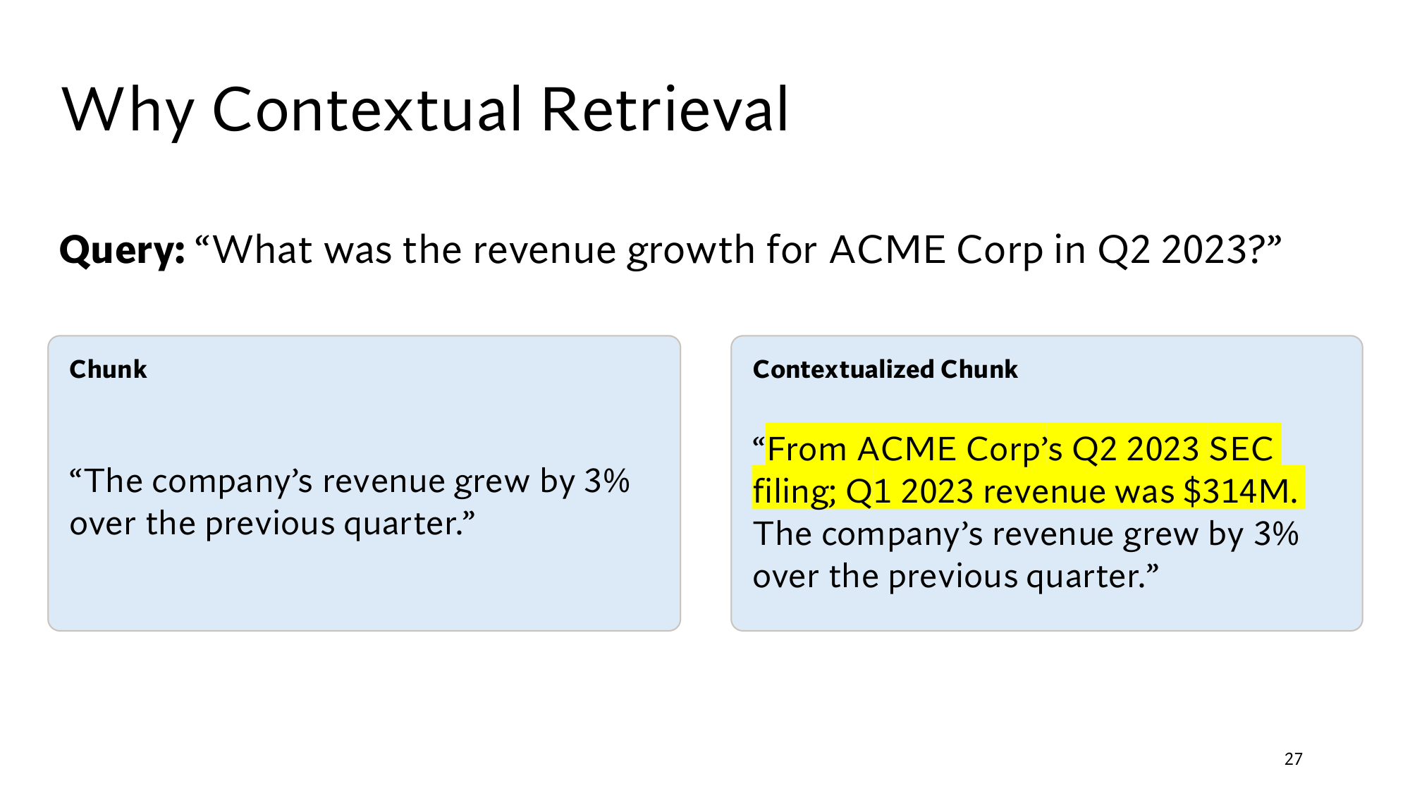
Take the example from the slides. The corpus holds the Q2 2023 quarterly filings of 50 companies, one per company. 50 companies is my example Almost every filing contains this line: The company’s revenue grew by X% over the previous quarter. The query is What was the revenue growth for ACME Corp in Q2 2023? ACME’s filing names the company and the quarter at the very top, so the chunk with the answer contains neither ACME nor Q2 2023.
Now count with lesson 2’s : how many of the query’s words also appear in the chunk. In lesson 2 the queue log scored 2, because it contained office and hour. After removing such as what, was, the, for and in, the query keeps 6 words: revenue, growth, ACME, Corp, Q2 and 2023. The ACME chunk contains only revenue, because it says grew, not growth. So it scores 1, and so do the other 49 chunks. my count
Think first
All 50 chunks score 1, and chunks with equal scores come out in random order. The retriever returns the top 20. How often does the ACME chunk make the top 20?
Show the answer
With a tie, the ACME chunk is equally likely to land in any of the 50 places. 20 of those places are in the top 20, so the chance is 20 ÷ 50 = 0.4, or 40%. The other 60% of the time the right chunk stays out of the top 20.
So the answer is in the corpus, yet the retriever misses it 60% of the time. An embedding does not save it either, because the embedding model reads only the chunk’s text. That text never mentions ACME, so the vector cannot carry anything about ACME.
Lesson 7’s keeps metadata with each chunk, but nobody will write metadata by hand for 60,000 chunks.
2Contextual retrieval: an LLM writes a context in front of each chunk
Contextual retrieval puts a short context in front of each chunk, written by an LLM that has read the whole document. Anthropic published the method in 2024. It runs four steps at , before any query arrives:
For each chunk, give the LLM the whole document and that chunk.
The LLM writes a short context for the chunk, 50 to 100 tokens long.
Put that context in front of the chunk. The new text is called a contextualized chunk.
Embed the contextualized chunk, and also add it to a word-based index, which comes in lesson 11.
For the ACME chunk, the LLM writes this context. The coloured part is the LLM’s, and the rest is the original chunk:
From ACME Corp’s Q2 2023 SEC filing; Q1 2023 revenue was $314M. The company’s revenue grew by 3% over the previous quarter.
Stanford’s slide: the query at the top, the bare chunk on the left, and the same chunk with the yellow context on the right. Click the image to open it at full size.
Think first
The query’s 6 words are revenue, growth, ACME, Corp, Q2 and 2023. What is the contextualized chunk’s word overlap score now? What will the other companies’ contextualized chunks score?
Show the answer
The ACME chunk scores 5: revenue, ACME, Corp, Q2 and 2023. Growth is still missing. The other companies’ contexts carry their own names, so they score at most 3: revenue, Q2 and 2023. my count
With the context added, the ACME chunk breaks out of the 49-way tie and goes straight to the top. The embedding model now also gets a text that contains ACME and Q2 2023.
Anthropic’s results: failed retrievals@20
Anthropic measured the method on real data. Assume each query has one right chunk. Then failed retrievals@20 is the percentage of queries whose right chunk did not make the top 20. The smaller this number, the better.
The drop in the third row is easiest to see on 1,000 queries:
With plain chunks, 5.7% × 1,000 = 57 queries fail.
With contextualized chunks, 3.7% × 1,000 = 37 queries fail.
57 − 37 = 20 queries are saved, and 20 ÷ 57 = 0.35. So failures fell by 35%.
The failure rate fell by only 2 points, from 5.7 to 3.7, yet failures fell by 35%. The drop in points is 5.7 − 3.7, and the percentage drop divides that by the starting value, 5.7. Add the word-based index as well, and failures fall to 2.9%, which is (5.7 − 2.9) ÷ 5.7 = 0.49, about half. How to merge the two indexes’ lists comes in lesson 14.
The cost comes at indexing time: one LLM call per chunk, and the whole document in every call. With 60,000 chunks, that is 60,000 calls. There is no extra cost at query time, because the context is already in the index. There is also a risk: if the LLM writes a wrong context, that mistake stays in the index.
3Late chunking: encode the whole document first, then average each chunk
LLM calls are expensive, so the next question is whether the encoder alone can supply the context. Lesson 7’s builds each token’s vector from the words around it. There, late had the vector [0.1, 0.9] in one sentence and [0.9, 0.1] in the other. But the encoder only sees the text it is given.
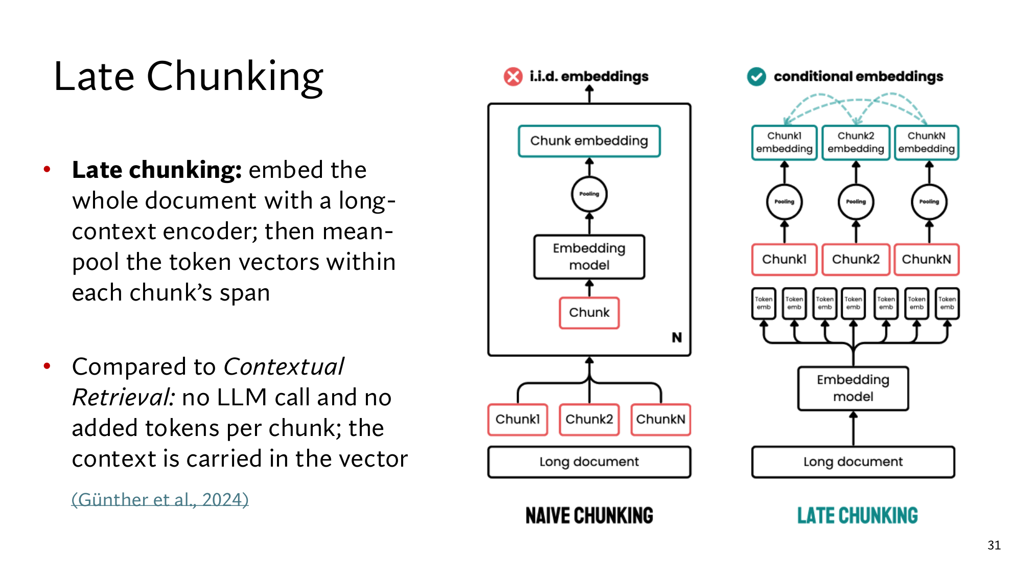
The usual method gives the encoder only the chunk: cut first, then encode each chunk on its own. This is called naive chunking. The chunk’s tokens know nothing about the rest of the document.
Late chunking reverses the order: the encoder reads the whole document first, and the cutting happens afterwards.
Feed the whole document into a long-context encoder, an encoder that can read a very long text in one go, such as 8,192 tokens, about 10 pages. from the paper
The encoder returns a vector for every token, and every vector is built with the whole document in view.
Average the token vectors inside each chunk. That average is the chunk’s vector.
This average is lesson 7’s , for example [0.9, 0.1], [0.7, 0.3] and [0.8, 0.2] give [0.8, 0.2]. The cutting happens after encoding, that is, late, hence the name.
Take a small document: CS 329Z project milestone policy. It is due Week 6. The second chunk is It is due Week 6. In each vector, the first number says how much the text is about the project milestone, and the second how much it is about homework. my numbers
Token
Naive: chunk alone
Late: whole document
It
[0.5, 0.5]
[0.9, 0.1]
is
[0.5, 0.5]
[0.8, 0.2]
due
[0.6, 0.4]
[0.9, 0.1]
Week
[0.4, 0.6]
[0.9, 0.1]
6
[0.5, 0.5]
[1.0, 0.0]
Mean pooling
[0.5, 0.5]
[0.9, 0.1]
The last row works out like this:
Naive, first number: (0.5 + 0.5 + 0.6 + 0.4 + 0.5) ÷ 5 = 2.5 ÷ 5 = 0.5. The second number is also 0.5.
In the naive version, It cannot tell whether the text is about the milestone or about homework, so the vector sits in the middle. In the late version, the encoder also read the first sentence, so every token leans towards the milestone.
Take the query When is the project milestone due? with the vector [0.95, 0.05]. Lesson 3’s divides the dot product by the product of the two lengths, as in 0.74 ÷ (0.82 × 0.91) = 0.99. The cosine with the naive chunk takes three steps:
For the late chunk [0.9, 0.1], the same arithmetic gives 0.86 ÷ (0.951 × 0.906) = 1.00. The late chunk points almost exactly the way the query does, while the naive chunk stays at 0.74.
Think first
Now take a homework query with the vector [0.05, 0.95]. Work out its cosine with the naive chunk [0.5, 0.5] and with the late chunk [0.9, 0.1]. What weakness of the naive chunk shows up?
The naive chunk gives 0.74 for both queries, so the milestone chunk ranks just as high for the homework question. my query
Stanford’s slide: naive chunking in the middle, and late chunking on the right.
In the paper, with chunks of 256 tokens, late chunking raised the average score from 52.2 to 54.0. This is a ranking score from 0 to 100, which lesson 13 opens up. The gain is largest for the smallest chunks, because a small chunk loses the most context.
4Comparing the two methods: context in the text or in the vector
The two methods keep the context in different places: contextual retrieval writes it into the chunk’s text, and late chunking keeps it only in the vector. The other differences follow from this:
Contextual retrieval
Late chunking
Who supplies the context
An LLM, by writing text
The encoder, inside the vectors
Indexing cost
One LLM call per chunk
One encoder run per document
Does the chunk get longer?
Yes, by 50–100 tokens
No
Helps a word-based index
Yes, the new words are in the text
No
The ACME query shows the difference directly. After late chunking, the chunk’s text still does not contain ACME, so its word overlap score stays at 1. So only contextual retrieval helps a word-based index, while both help embeddings. Late chunking also has a limit: the whole document must fit within the encoder’s length limit, or the context gets cut again.
Think first
The corpus is very large, the budget for LLM calls is small, chunks are 64 tokens, and the retriever uses embeddings only. Which method do you pick? What if the retriever is a word-based index only?
Show the answer
Late chunking. It needs no LLM call, and its gain is largest on small chunks. On a word-based index alone, late chunking does nothing, because its context never reaches the text. Then pick contextual retrieval.
What the dense version adds
The dense version contains this whole lesson, followed by 5 more steps that take you to the level of the Stanford slides:
Step 5: Anthropic’s full pipeline, the prompt, the metric, the cost, and 1.9% with reranking.
Step 6: late chunking from the inside: i.i.d. and conditional embeddings, attention, and the paper’s pooling formula.
Step 7: the paper’s results, the chunk-size charts, and long late chunking.
Step 8: both methods on the same ACME example, with the paper’s cosine numbers.
Step 9: all six Stanford slides of this part, which you read yourself.
Cutting makes a chunk lose its context. The ACME chunk ended up tied with 49 other chunks, and it makes the top 20 only 40% of the time.
Contextual retrieval has an LLM write a context in front of each chunk. Failed retrievals@20 fell from 5.7% to 3.7%, and to 2.9% with a word-based index.
Late chunking encodes the whole document first, then averages each chunk’s token vectors. It needs no LLM call, but the context lives only in the vector.
New terms in this lesson
Context loss
After cutting, a chunk can no longer say which document or topic it belongs to. For example, The company’s revenue grew by 3% does not name the company.
Contextual retrieval
Indexing each chunk with a 50–100 token context, written by an LLM, placed in front of it. For example, adding From ACME Corp’s Q2 2023 SEC filing.
Failed retrievals@20
When each query has one right chunk, the percentage of queries whose right chunk is not in the top 20. Smaller is better. For example, 29 failures in 1,000 queries is 2.9%.
Naive chunking
Cutting first, then encoding each chunk on its own. Then the vector of It is due Week 6 stays at [0.5, 0.5].
Late chunking
Encoding the whole document first, then mean pooling each chunk’s token vectors. Then the vector of It is due Week 6 becomes [0.9, 0.1].
Long-context encoder
An encoder that can read a very long text in one go. For example, 8,192 tokens, about 10 pages.